35 Collapsing Categories
35.1 Collapsing Categories
There are times, especially when you have a lot of levels in a categorical variable, that it will be beneficial for you to combine some of them. This practice is in some ways similar to what we saw in Chapter 16 about cleaning categorical variables, but here we are doing it for performance reasons.
Essentially what we are working on, is trying to combine many levels to get higher performance and interpretability
this has two prongs
- there aren’t enough observations here, let us combine them
- these levels are similar
- expert knowledge
- inferred from data
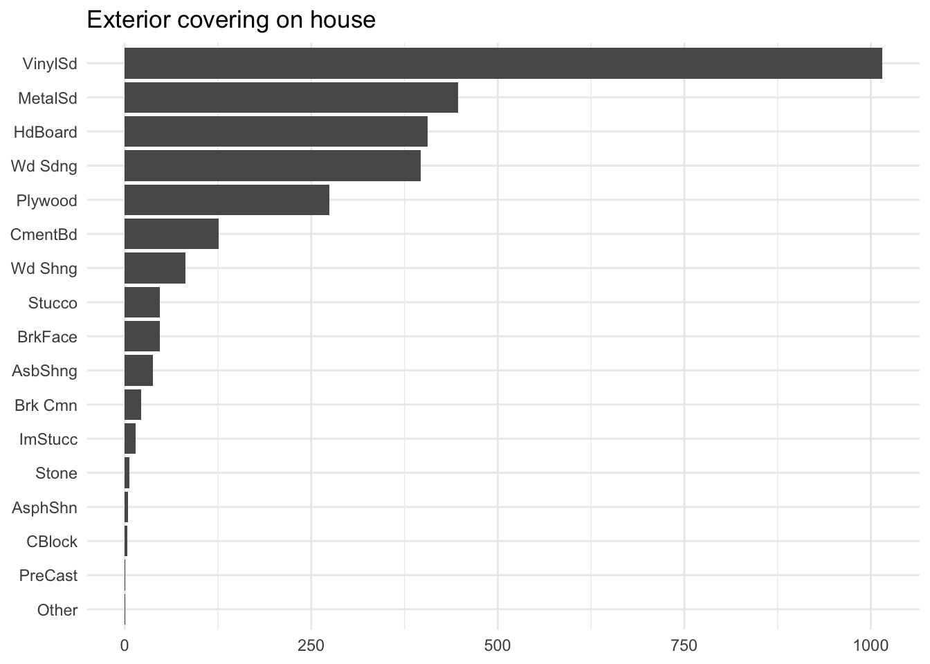
The first issue can be quite a common one. See the below distribution as an example
The proportion of how often each level appears is quite stark, to the point where 4 of them happen less than 10 times, which is not a lot considering the most frequent level occurs over 1000 times.
For some methods such as Dummy Encoding, having these infrequent levels would not do us much good, and may even make things worse. Having a level be so infrequent increases its likelihood of being uninformative. This is where collapsing can come into play. The method takes the most infrequent levels and combines them into one, typically called "other".
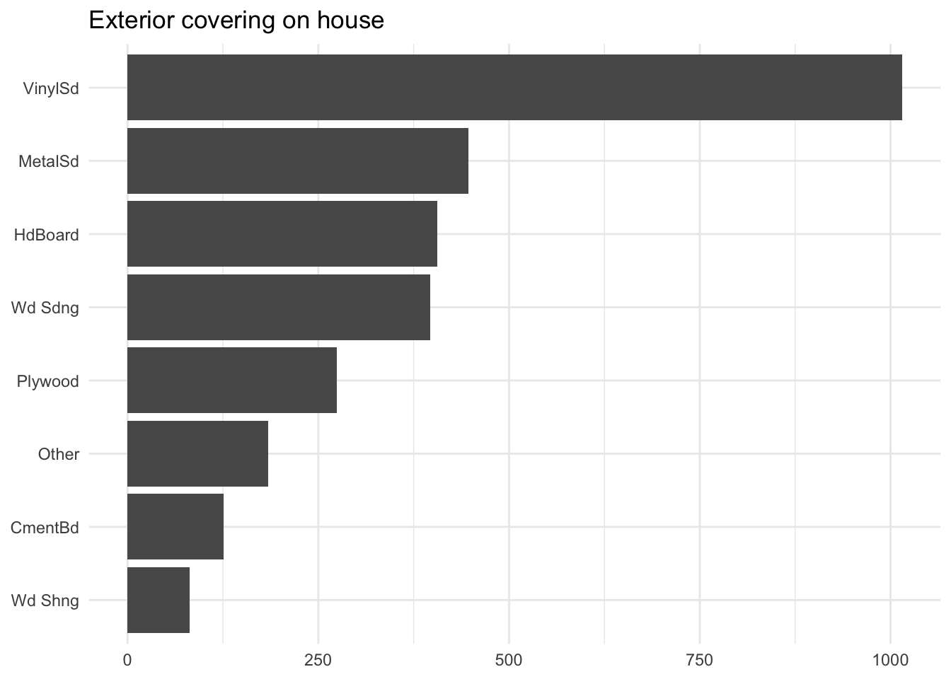
Above we see how that is done. We took all the levels that appeared less than 2.5% of the time and combined them into a new level called "other". This value threshold will off cause depend on many things and is a good candidate for tuning. And we don’t have to do it as a percentage, we might as well do it based on counts. Collapsing anything with less than 10 occurrences.
This method can give pretty good results. But is by nature very crude. We are more than likely to combine levels that have nothing to do with each other than their low frequency. This will sometimes be inefficient, and while it has straightforward explainability due to its simple nature it can be hard to argue for its approach to shareholders.
This is where the other type of collapsing comes in. These methods use a little more information about the data, in the hopes that the collapsing will be more sensible. We will describe two of them here. First is the model-based approach. You can imagine that we fit a small model, such as a decision tree on the categorical variable, using a sensible outcome. This outcome could the the real outcome of our larger modeling problem. then we let the decision tree run, and the way the tree splits the data is how we combine the levels.
This is done below as an example:
$Exterior_2nd_1
[1] "AsbShng" "AsphShn" "CBlock"

$Exterior_2nd_2
[1] "Brk Cmn"

$Exterior_2nd_3
[1] "Stone"   "Stucco"  "Wd Sdng"

$Exterior_2nd_4
[1] "MetalSd" "Wd Shng"

$Exterior_2nd_5
[1] "HdBoard" "Plywood"

$Exterior_2nd_6
[1] "BrkFace"

$Exterior_2nd_7
[1] "VinylSd"

$Exterior_2nd_8
[1] "CmentBd"

$Exterior_2nd_9
[1] "ImStucc" "Other"   "PreCast"
And it isn’t super hard to see that these make sense. “Asbestos Shingles” and “Asphalt Shingles” got paired, as did “Metal Siding” and “Wood Siding”, and “Hard Board” and “Plywood”. These are of course only linked because they appear similar when looking at the sale price. But We are likely able to reason better about these new labels than before.
CautionTODO
add a plot of the tree
When to stop growing the is still something that we can and should tune. Too small of a tree and we collapse levels that should be different, too large a tree and we don’t collapse things that should have been collapsed.
Another interesting method is when we use the levels themselves to decide how to do the collapsing. Using string distances between the levels. Hence similar levels will be collapsed together.
CautionTODO
Also talk about min-hash encoder https://arxiv.org/abs/1907.01860 https://arxiv.org/abs/1806.00979
$AsbShng
[1] "AsbShng" "AsphShn" "Wd Sdng" "Wd Shng"

$`Brk Cmn`
[1] "Brk Cmn" "BrkFace" "PreCast"

$CBlock
[1] "CBlock"  "ImStucc" "Other"   "Stone"   "Stucco"

$CmentBd
[1] "CmentBd"

$HdBoard
[1] "HdBoard"

$MetalSd
[1] "MetalSd" "VinylSd"

$Plywood
[1] "Plywood"
CautionTODO
add a plot of what happens here
This doesn’t use the data at all, and the results reflect that. The distance will again have to be used for best results, and there are quite a few different types of ways to calculate string distance. The choices will sometimes matter a lot and should be investigated before use for best results.
The string distance collapsing method does in some ways feel like a cleaning method like we saw in Chapter 16 about cleaning categorical variables. Having many levels in a freeform state will often lead to misspellings or other slight variations. String distances are a great way to deal with those types of problems. It is recommended that you always look at the resulting mappings to make sure they are created correctly, or good enough.
Some data is naturally hierarchical, and if we have this type of data and we want to collapse, we can take advantage of that and collapse according to the hierarchies.
Collapsing categorical levels is not without risk, and each application should be monitored and checked to make sure we don’t do anything bad. In many ways, this is quite a manual process and luckily the results are very easy to validate.
Unseen levels will have to be treated on a method-to-method basis. Tree-based collapsing will not be able to handle unseen levels as they are not part of the tree at all. On the other hand, it is possible to handle unseen levels on the string distance method as you just need to calculate the distances. With the caveat that some strings could be the same distance away from multiple levels.
35.2 Pros and Cons
35.2.1 Pros
- Easy to perform and verify
- Computationally fast
35.2.2 Cons
- Must be tuned
- Can produce counterintuitive results
35.3 R Examples
Methods to collapse categorical levels can be found in the recipes package with step_other() and the embed package in step_collapse_cart() and step_collapse_stringdist().
CautionTODO
find a better data set for examples
Othering can be done using the step_other() function, it uses the argument threshold to determine the cutoff used to turn levels into "other" or not.
library(recipes)
library(embed)

data(ames, package = "modeldata")

rec_other <- recipe(Sale_Price ~ Exterior_2nd, data = ames) |>
  step_other(Exterior_2nd, threshold = 0.1) |>
  prep()

rec_other |>
  bake(new_data = NULL)
# A tibble: 2,930 × 2
Exterior_2nd Sale_Price
<fct> <int>
1 other 215000
2 VinylSd 105000
3 Wd Sdng 172000
4 other 244000
5 VinylSd 189900
6 VinylSd 195500
7 other 213500
8 HdBoard 191500
9 other 236500
10 VinylSd 189000
# ℹ 2,920 more rowsselecting a higher threshold turns more levels into "other".
rec_other <- recipe(Sale_Price ~ Exterior_2nd, data = ames) |>
  step_other(Exterior_2nd, threshold = 0.5) |>
  prep()

rec_other |>
  bake(new_data = NULL)
# A tibble: 2,930 × 2
Exterior_2nd Sale_Price
<fct> <int>
1 other 215000
2 VinylSd 105000
3 other 172000
4 other 244000
5 VinylSd 189900
6 VinylSd 195500
7 other 213500
8 other 191500
9 other 236500
10 VinylSd 189000
# ℹ 2,920 more rowsfor the more advanced methods, we turn to the embed package. To collapse levels by their string distance, we use the step_collapse_stringdist(). By default, you control it with the distance argument.
rec_stringdist <- recipe(Sale_Price ~ Exterior_2nd, data = ames) |>
  step_collapse_stringdist(Exterior_2nd, distance = 5) |>
  prep()

rec_stringdist |>
  bake(new_data = NULL)
# A tibble: 2,930 × 2
Exterior_2nd Sale_Price
<fct> <int>
1 Plywood 215000
2 MetalSd 105000
3 AsbShng 172000
4 Brk Cmn 244000
5 MetalSd 189900
6 MetalSd 195500
7 CmentBd 213500
8 HdBoard 191500
9 CmentBd 236500
10 MetalSd 189000
# ℹ 2,920 more rowsUnsurprisingly, there are almost a dozen different ways to calculate the distance between two strings. Most are supported and can be changed using the method argument, and further controlled using the options argument.
rec_stringdist <- recipe(Sale_Price ~ Exterior_2nd, data = ames) |>
  step_collapse_stringdist(Exterior_2nd,
                           distance = 0.75,
                           method = "cosine",
                           options = list(q = 2)) |>
  prep()

rec_stringdist |>
  bake(new_data = NULL)
# A tibble: 2,930 × 2
Exterior_2nd Sale_Price
<fct> <int>
1 Plywood 215000
2 MetalSd 105000
3 AsbShng 172000
4 Brk Cmn 244000
5 MetalSd 189900
6 MetalSd 195500
7 CmentBd 213500
8 HdBoard 191500
9 CmentBd 236500
10 MetalSd 189000
# ℹ 2,920 more rowsLastly, we have the tree-based method, this is done using the step_collapse_cart() function. For this to work, you need to select an outcome variable using the outcome argument. With cost_complexity and min_n as arguments to change the shape of the tree.
rec_cart <- recipe(Sale_Price ~ Exterior_2nd, data = ames) |>
  step_collapse_cart(Exterior_2nd, outcome = vars(Sale_Price)) |>
  prep()

rec_cart |>
  bake(new_data = NULL)
# A tibble: 2,930 × 2
Exterior_2nd Sale_Price
<fct> <int>
1 Exterior_2nd_5 215000
2 Exterior_2nd_7 105000
3 Exterior_2nd_3 172000
4 Exterior_2nd_6 244000
5 Exterior_2nd_7 189900
6 Exterior_2nd_7 195500
7 Exterior_2nd_8 213500
8 Exterior_2nd_5 191500
9 Exterior_2nd_8 236500
10 Exterior_2nd_7 189000
# ℹ 2,920 more rows