27 GLMM Encoding
27.1 GLMM Encoding
Generalized linear mixed models (GLMM) encoding Pargent et al. (2022) follows as an extension to target encoding which is laid out in detail in Chapter 23.
A hierarchical generalized linear model is fit, using no intercept.
When applying target encoding, some classes have different numbers of observations associated with them.
The "horse" class only has 1 observation in this data set, how confident are we that the mean calculated from this value is as valid as the mean that was calculated over the 3 values for the "cat" class?
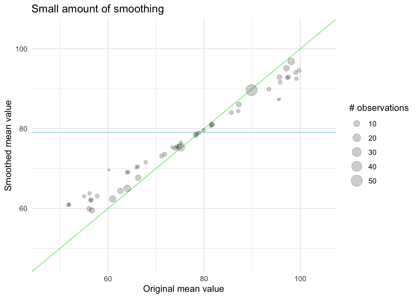
Knowing that the global mean of the target is our baseline when we have no information. We can combine the level mean with the global mean, in accordance with how many observations we observe. If we have a lot of observations at a level, we will let the global mean have little influence, and if there are fewer observations we will let the global mean have a higher influence.
We can visualize this effect in the following charts. First, we have an example of what happens with a smaller amount of smoothing. The points are mostly along the diagonal. Remember that if we didn’t do this, all the points would be along the diagonal regardless of their size.

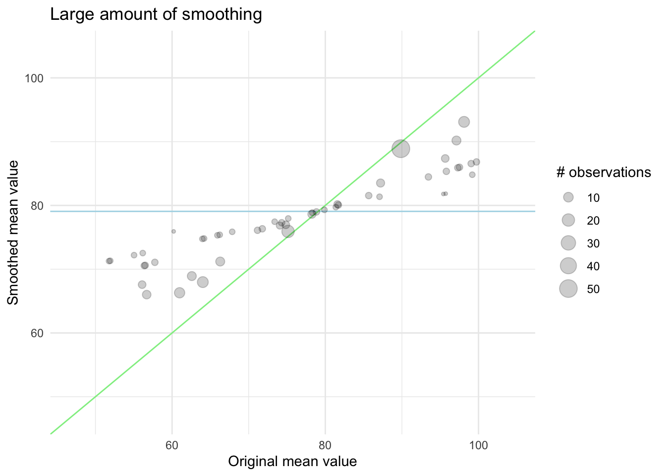
In this next chart, we see the effect of a higher amount of smoothing, now the levels with fewer observations are pulled quite a bit closer to the global mean.

The exact way this is done will vary from method to method, and the strength of this smoothing can and should properly be tuned as there isn’t an empirical best way to choose it.
The big benefit is that by fitting a hierarchical generalized linear model is fit, using no intercept is that it will handle the amount of smoothing for us. Giving us a method that handles smoothing, using a sound statistical method, without needed a hyperparameter.
27.2 Pros and Cons
27.2.1 Pros
- No hyperparameters to tune, as shrinkage is automatically done
- Can deal with categorical variables with many levels
- Can deal with unseen levels in a sensible way
27.2.2 Cons
- Can be prone to overfitting
27.3 R Examples
find a better data set
We apply the smoothed GLMM encoder using the step_lencode_mixed() step.
library(recipes)
library(embed)

data(ames, package = "modeldata")

rec_target_smooth <- recipe(Sale_Price ~ Neighborhood, data = ames) |>
  step_lencode_mixed(Neighborhood, outcome = vars(Sale_Price)) |>
  prep()

rec_target_smooth |>
  bake(new_data = NULL)
# A tibble: 2,930 × 2
Neighborhood Sale_Price
<dbl> <int>
1 145156. 215000
2 145156. 105000
3 145156. 172000
4 145156. 244000
5 190633. 189900
6 190633. 195500
7 322591. 213500
8 322591. 191500
9 322591. 236500
10 190633. 189000
# ℹ 2,920 more rowsAnd we can pull out the values of the encoding like so.
rec_target_smooth |>
  tidy(1)
# A tibble: 29 × 4
level value terms id
<chr> <dbl> <chr> <chr>
1 North_Ames 145156. Neighborhood lencode_mixed_Bp5vK
2 College_Creek 201769. Neighborhood lencode_mixed_Bp5vK
3 Old_Town 124154. Neighborhood lencode_mixed_Bp5vK
4 Edwards 131021. Neighborhood lencode_mixed_Bp5vK
5 Somerset 229563. Neighborhood lencode_mixed_Bp5vK
6 Northridge_Heights 321519. Neighborhood lencode_mixed_Bp5vK
7 Gilbert 190633. Neighborhood lencode_mixed_Bp5vK
8 Sawyer 136956. Neighborhood lencode_mixed_Bp5vK
9 Northwest_Ames 188401. Neighborhood lencode_mixed_Bp5vK
10 Sawyer_West 184085. Neighborhood lencode_mixed_Bp5vK
# ℹ 19 more rows27.4 Python Examples
We are using the ames data set for examples. {category_encoders} provided the GLMMEncoder() method we can use.
from feazdata import ames
from sklearn.compose import ColumnTransformer
from category_encoders.glmm import GLMMEncoder

ct = ColumnTransformer(
    [('glmm', GLMMEncoder(), ['MS_Zoning'])],
    remainder="passthrough")

ct.fit(ames, y=ames[["Sale_Price"]].values.flatten())
ColumnTransformer(remainder='passthrough',
transformers=[('glmm', GLMMEncoder(), ['MS_Zoning'])])In a Jupyter environment, please rerun this cell to show the HTML representation or trust the notebook. On GitHub, the HTML representation is unable to render, please try loading this page with nbviewer.org.
ColumnTransformer(remainder='passthrough',
transformers=[('glmm', GLMMEncoder(), ['MS_Zoning'])])['MS_Zoning']
GLMMEncoder()
['MS_SubClass', 'Lot_Frontage', 'Lot_Area', 'Street', 'Alley', 'Lot_Shape', 'Land_Contour', 'Utilities', 'Lot_Config', 'Land_Slope', 'Neighborhood', 'Condition_1', 'Condition_2', 'Bldg_Type', 'House_Style', 'Overall_Cond', 'Year_Built', 'Year_Remod_Add', 'Roof_Style', 'Roof_Matl', 'Exterior_1st', 'Exterior_2nd', 'Mas_Vnr_Type', 'Mas_Vnr_Area', 'Exter_Cond', 'Foundation', 'Bsmt_Cond', 'Bsmt_Exposure', 'BsmtFin_Type_1', 'BsmtFin_SF_1', 'BsmtFin_Type_2', 'BsmtFin_SF_2', 'Bsmt_Unf_SF', 'Total_Bsmt_SF', 'Heating', 'Heating_QC', 'Central_Air', 'Electrical', 'First_Flr_SF', 'Second_Flr_SF', 'Gr_Liv_Area', 'Bsmt_Full_Bath', 'Bsmt_Half_Bath', 'Full_Bath', 'Half_Bath', 'Bedroom_AbvGr', 'Kitchen_AbvGr', 'TotRms_AbvGrd', 'Functional', 'Fireplaces', 'Garage_Type', 'Garage_Finish', 'Garage_Cars', 'Garage_Area', 'Garage_Cond', 'Paved_Drive', 'Wood_Deck_SF', 'Open_Porch_SF', 'Enclosed_Porch', 'Three_season_porch', 'Screen_Porch', 'Pool_Area', 'Pool_QC', 'Fence', 'Misc_Feature', 'Misc_Val', 'Mo_Sold', 'Year_Sold', 'Sale_Type', 'Sale_Condition', 'Sale_Price', 'Longitude', 'Latitude']
passthrough
ct.transform(ames) glmm__MS_Zoning ... remainder__Latitude
0 55180.830 ... 42.054
1 338.691 ... 42.053
2 55180.830 ... 42.053
3 55180.830 ... 42.051
4 55180.830 ... 42.061
... ... ... ...
2925 55180.830 ... 41.989
2926 55180.830 ... 41.988
2927 55180.830 ... 41.987
2928 55180.830 ... 41.991
2929 55180.830 ... 41.989
[2930 rows x 74 columns]