Non-Negative Matrix Factorization (NMF) is a method quite similar to Principal Component Analysis. PCA aims to create a transformation that maximizes the variance of the resulting variables, while making them uncorrelated. NMF, on the other hand, is a decomposition where the loadings are required to be non-negative.
CautionTODO
Add a diagram showing the matrix decomposition.
All the factor loadings are calculated at once, which is in contrast to PCA, where each component is calculated one by one. This difference comes with some different effects. It means that there isn’t an ordering or ranking in the resulting features. In PCA, the first output feature will be the same (up to a sign) no matter if you ask for 1 PC or 10 PCs. This is not the case for NMF, as the signal is spread across all the output features. The amount of signal contained in each feature will be quasi-reversely correlated with the number of features. The number of components is thus a hyperparameter you want to tune, trying to find a number that pulls out useful signals in the data without trying to pack too much information into too few components.
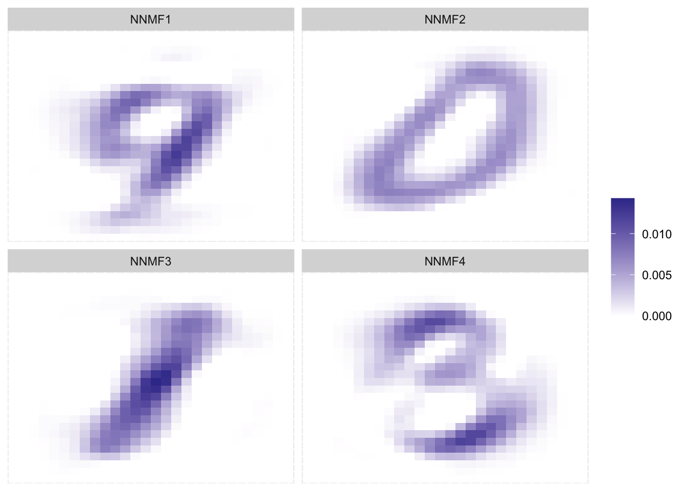
Below is an example where we apply NMF to the MNIST data set, asking for 4 components. Each pixel is treated as a predictor, and the colors show the factor loadings for each component. Visually showing which part of the image it is activated from.
The keras package is deprecated. Please use the keras3 package instead.
Alternatively, to continue using legacy keras, call `py_require_legacy_keras()`.
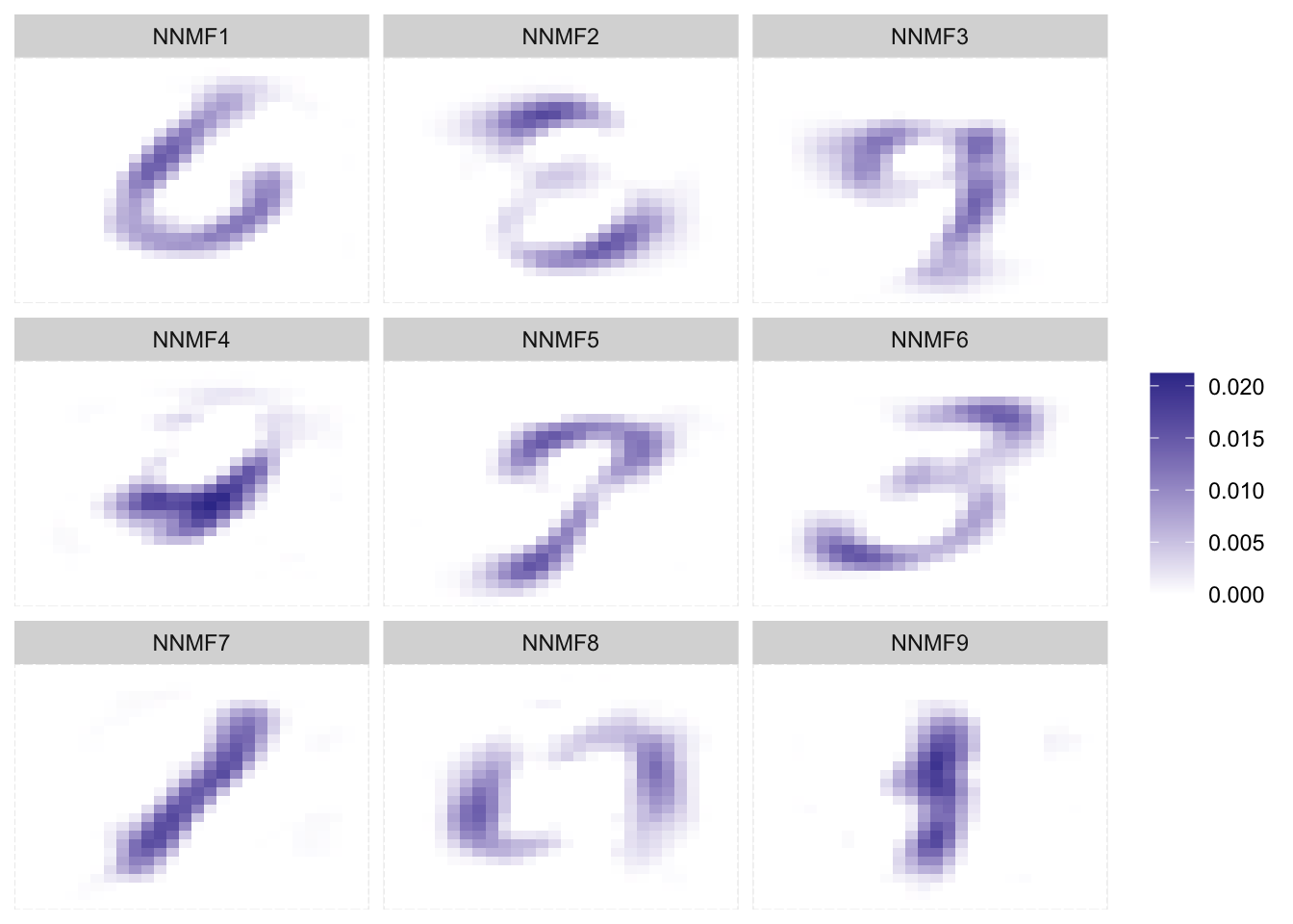
If we instead increase the number of components to 9, We see that each component pulls more and different shapes than before.
Figure 71.2: NMF applied to all of MNIST
This is also a good time to note that many implementations of NMF depend on the initialization,
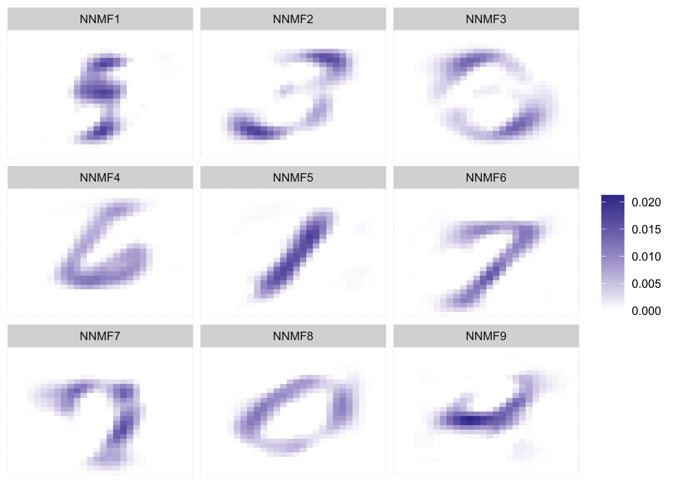
Figure 71.3: NMF applied to all of MNIST
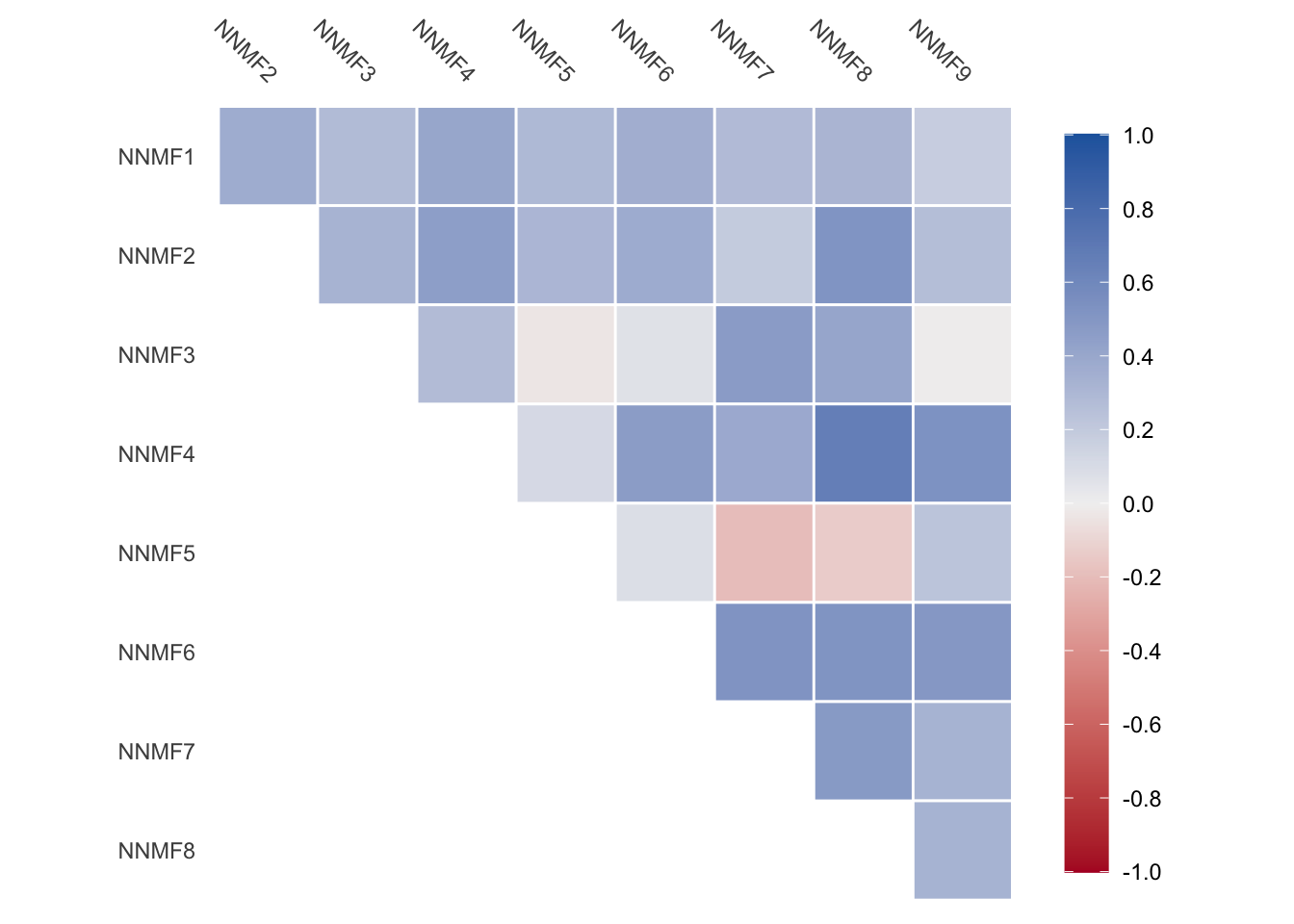
Note that the features are correlated, as it wasn’t a restriction that they would be.
Warning: Using `size` aesthetic for lines was deprecated in ggplot2 3.4.0.
ℹ Please use `linewidth` instead.
ℹ The deprecated feature was likely used in the corrr package.
  Please report the issue at <https://github.com/tidymodels/corrr/issues>.
Figure 71.4: Non-zero correlation between all features.
Creating the decomposition is computationally harder, and more computationally expensive than PCA, An approximate implementation is often used to mitigate those facts. which sadly means that the algorithms are able to find local maxima, But not guaranteed to find global maxima. This leads to the solutions not being unique and may need to run multiple times with different seeds to find a better maximum.
There are a couple of restrictions on the data to which NMF can be applied. It only accepts numeric data, with no missing values, and no negative values. No missing values isn’t that bad of a restriction, as it is shared with most other dimensionality reduction methods. The non-negative restriction can be much more impactful. While the requirement that the input data is non-negative is a downside, it isn’t that big of a downside for many use cases, as non-negative data is quite common in many fields, as it represents counts and measurements quite well.
Since all the data is required to be non-negative and all the loading values are non-negative, We get quite nice interpretability as the different features don’t cancel each other out. Furthermore, some implementations are done to produce sparse loadings, making the interpretability even easier. The main downside of turning on sparsity is that we will need to find the right amount of sparsity to avoid decreases in performance.
71.2 Pros and Cons
71.2.1 Pros
More interpretable results
71.2.2 Cons
Data must be non-negative
Computationally expensive
Training depends on the seed
71.3 R Examples
We will be using the ames data set for these examples.