70  Independent Component Analysis

Independent Component Analysis (ICA) is a method quite similar to Principal Component Analysis. PCA aims to create a transformation that maximizes the variance of the resulting variables, while making them uncorrelated. ICA, on the other hand, aims to create variables that are statistically independent. Note that the ICA components are not assumed to be uncorrelated or orthogonal.

This allows ICA to pull out stronger signals in your data. It also doesn’t assume that the data is Gaussian.

One way to think about the difference between PCA and ICA, PCA can be used more effectively as a data compression technique, On the other hand, ICA helps uncover and separate the structure in the data itself.

The notion that ICA is a dimensionality reduction method is because the implementation of fastICA, which is commonly used, works incrementally.

ICA, much like PCA, requires that your data be normalized before it is applied.

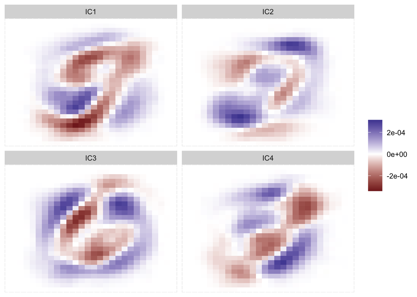
Below is an example of the principle components in actions. We took the MNIST database and performed ICA on the pixel values as predictors. First We apply it to the entire data set.

The keras package is deprecated. Use the keras3 package instead.
[1] 60000    28    28
── Attaching packages ────────────────────────────────────── tidymodels 1.4.1 ──
βœ” broom        1.0.10     βœ” recipes      1.3.1 
βœ” dials        1.4.2      βœ” rsample      1.3.1 
βœ” dplyr        1.1.4      βœ” tailor       0.1.0 
βœ” ggplot2      4.0.0      βœ” tidyr        1.3.1 
βœ” infer        1.0.9      βœ” tune         2.0.0 
βœ” modeldata    1.5.1      βœ” workflows    1.3.0 
βœ” parsnip      1.3.3      βœ” workflowsets 1.1.1 
βœ” purrr        1.1.0      βœ” yardstick    1.3.2 
── Conflicts ───────────────────────────────────────── tidymodels_conflicts() ──
βœ– purrr::discard()         masks scales::discard()
βœ– dplyr::filter()          masks stats::filter()
βœ– yardstick::get_weights() masks keras::get_weights()
βœ– dplyr::lag()             masks stats::lag()
βœ– recipes::step()          masks stats::step()

Faceted tile chart. Each chart corresponds to a different component. Early components show some shapes that might suggest numbers such as 6 or 7, later ones show less and less identifiable patterns.

ICA applied to all of MNIST

We clearly see some effects here. Remember that it isn’t important whether something is positive or negative, just that something is different than something else. there isn’t super strong signals, but it appears that we are capturing 7-ness in the first IC and 6-ness in the third IC. We notice that each IC appears

70.2 Pros and Cons

70.2.1 Pros

  • Can identify stronger signals

70.2.2 Cons

  • Sensitive to noise and outliers
  • Computationally intensive

70.3 R Examples

We will be using the ames data set for these examples.

library(recipes)
library(modeldata)

ames_num <- ames |>
  select(where(is.numeric))

{recipes} provides step_ica(), which is the standard way to perform ICA.

pca_rec <- recipe(~ ., data = ames_num) |>
  step_normalize(all_numeric_predictors()) |>
  step_ica(all_numeric_predictors())

pca_rec |>
  prep() |>
  bake(new_data = NULL) |>
  glimpse()
Rows: 2,930
Columns: 5
$ IC1 <dbl> 1.98722112, -0.19544103, 1.52173527, 1.70182755, -0.41432529, -0.3…
$ IC2 <dbl> 0.7781170, 0.9250619, 1.3102098, -0.1816165, -0.6315028, -0.747662…
$ IC3 <dbl> 0.37976490, -0.51412721, 0.80773773, -0.11337596, 0.64724658, 0.54…
$ IC4 <dbl> -0.115604620, 0.924486173, -0.788614494, -0.441096097, 0.394126431…
$ IC5 <dbl> 0.82127411, 0.57740102, 0.43923180, 0.81572982, -1.01902720, -1.06…

70.4 Python Examples