64 Periodic Splines
64.1 Periodic Splines
This chapter expands the idea we saw in the last chapter with the use of splines. These splines allow for different shapes of activation than we saw with trigonomic functions.
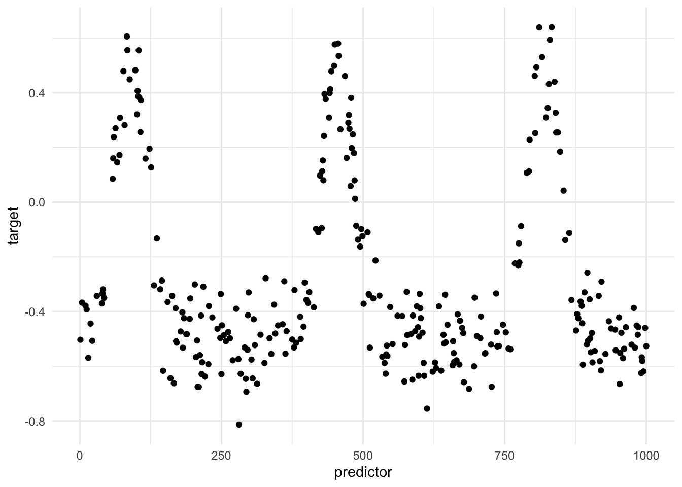
We will be using the same toy data set and see if we can improve on it.
This data has a very specific shape, and we will see if we can approcimate it with our splines.
First we fit a number of spline terms to our data using default arguments.
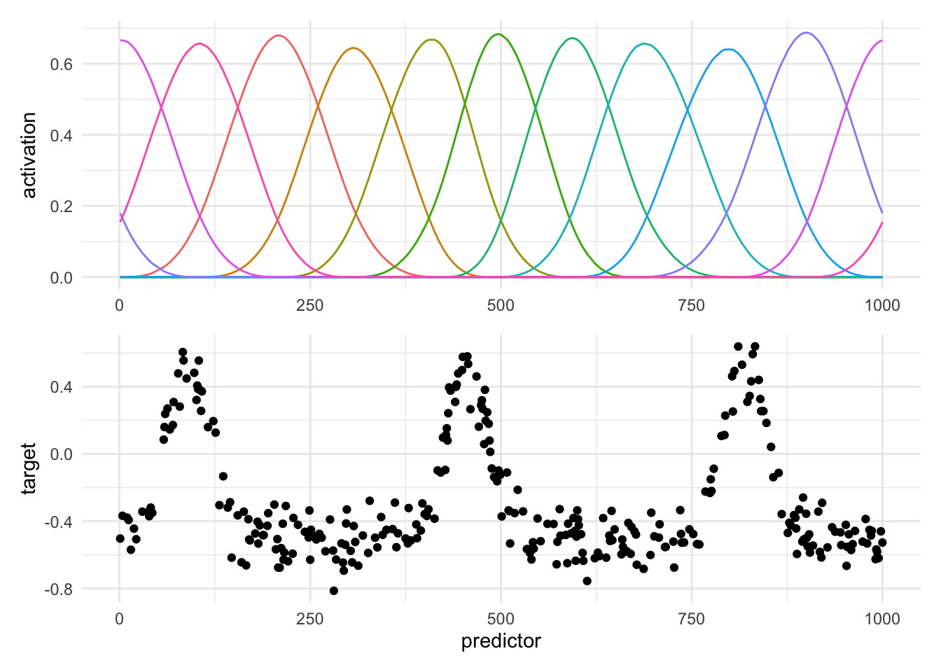
While it produces some fine splines they are neither well fitting or periodic. Let us make spline periodic and try to approcimate the period.
![Two stacked charts. Bottom: scatter plot showing periodic target data. Top: periodic B-spline basis with Boundary.knots set to [0, 365]. The spline curves now repeat every 365 units, matching the data's period. Multiple bell-shaped curves tile the space, each activating for a different phase of the cycle.](periodic-splines_files/figure-html/fig-periodic-spline-period-1.png)
We already see that something good is happening, The width of each bump is related to the number of degrees of freedom we have, lowering this value creates more wider bumps.
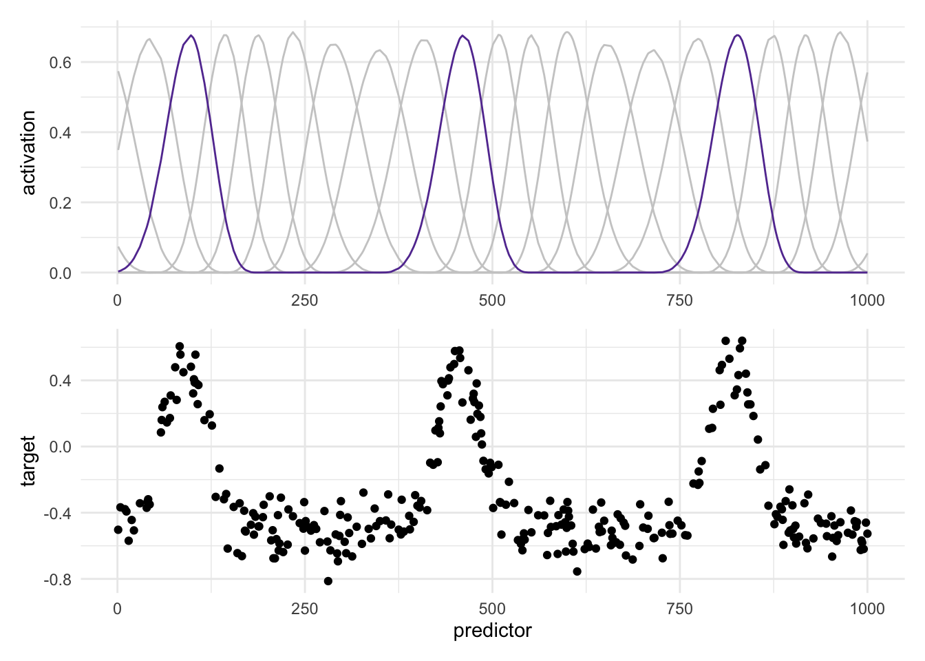
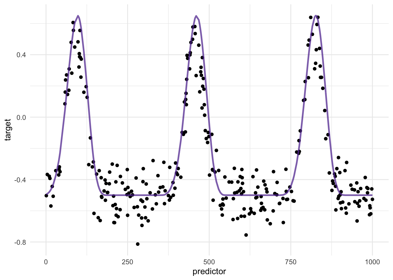
Now we got some pretty good traction. Pulling out the well performing spline term, we can translate it a bit to show how well it overlaps with our signal.
Note
While one spline term is highlighted here, It is important to note that the coverage of the splines makes sure that any signal is captured.
There are obviously some signals that can’t be captured using splines. Compared to sine curves they are much more flexible, with a number of different kinds, each with some room for customization. Any purely periodic signal can be captured in the next chapter.
64.2 Pros and Cons
64.2.1 Pros
- More flexible than sine curves
- Fairly interpretable
64.2.2 Cons
- Requires that you know the period
- Will create some unnecessary features
- Can’t capture all types of signal
64.3 R Examples
We will be using the animalshelter data set for this.
library(recipes)
library(animalshelter)

longbeach |>
  select(outcome_type, intake_date)
# A tibble: 29,787 × 2
outcome_type intake_date
<chr> <date>
1 euthanasia 2023-02-20
2 rescue 2023-10-03
3 euthanasia 2020-01-01
4 transfer 2020-02-02
5 rescue 2018-12-18
6 adoption 2024-10-18
7 euthanasia 2020-07-25
8 rescue 2019-06-12
9 rescue 2017-09-21
10 rescue 2024-12-15
# ℹ 29,777 more rowsThere are two steps in the recipes package that support periodic splines. Those are step_spline_b() and step_spline_nonnegative(), used for B-splines and Non-negative splines (also called M-Splines) respectively.
These functions have 2 main arguments controlling the spline itself, and 2 main arguments controlling its periodic behavior.
deg_free and degree controls the spline, changing the number of spline terms that are created, and the degrees of the piecewise polynomials respectively. The defaults for these functions tend to be a good starting point. To make these steps periodic, we need to set periodic = TRUE in options. Lastly, we can control the period and its shift with Boundary.knots in options. I find the easiest way to set this like this: c(0, period) + shift.
spline_rec <- recipe(outcome_type ~ intake_date, data = longbeach) |>
  step_mutate(intake_date = as.integer(intake_date)) |>
  step_spline_b(
    intake_date,
    options = list(periodic = TRUE, Boundary.knots = c(0, 365) + 50)
  )

spline_rec |>
  prep() |>
  bake(new_data = NULL)
# A tibble: 29,787 × 11
outcome_type intake_date_01 intake_date_02 intake_date_03 intake_date_04
<fct> <dbl> <dbl> <dbl> <dbl>
1 euthanasia 0 0 0 0
2 rescue 0 0 0 0
3 euthanasia 0 0 0 0
4 transfer 0 0 0 0
5 rescue 0 0 0 0
6 adoption 0 0 0 0
7 euthanasia 0 0.0154 0.437 0.512
8 rescue 0.176 0.682 0.142 0
9 rescue 0 0 0 0.0131
10 rescue 0 0 0 0
# ℹ 29,777 more rows
# ℹ 6 more variables: intake_date_05 <dbl>, intake_date_06 <dbl>,
# intake_date_07 <dbl>, intake_date_08 <dbl>, intake_date_09 <dbl>,
# intake_date_10 <dbl>
CautionTODO
Find dataset where the predictor is naturally numeric.