Uniform Manifold Approximation and Projection (UMAP) is another method that takes high-dimensional data and embeds it into a lower-dimensional space. This method is in the same category of encoders as autoencoders and ISOMAP, as they allow for non-linear compression of the data. This method got popular in part because of how fast it runs, and because people tend to like the visualization it provides.
UMAP is an iterative stochastic method. It works by doing the following steps:
Use spectral embedding to embed points in a low-dimensional space
Calculate similarity scores between all pairs of points based on the original data set
Randomly samples a pair of points based on their similarity scores
Flips a coin to decide which of the pair of points to focus on
Randomly picks a non-neighbor point to move away from
Moves the selected point towards its neighbor and away from its non-neighbor
Repeat 3-6
Beyond arguments such as n_epochs, which would determine how long to run this algorithm for, and n_components to determine the number of components to return. There are 3 main hyperparameters: n_neighbors, min_dist, and metric. n_neighbors determines how many points are considered neighbors. A point counts as its own neighbor. Lower values lead to a local view. min_dist determines how close points are allowed to be to each other in the low-dimensional space. metric determines how distances are calculated in the input data: euclidean, manhattan, jaccard, etc. There are many more arguments for UMAP, It is quite a flexible method that has been used in many fields.
One of the consequences of the algorithm is that only local distances matter in our embedding. That is to say that points that are close together in our embedding are also close together in the original data, but each component doesn’t carry any actionable information beyond its ability to separate points.
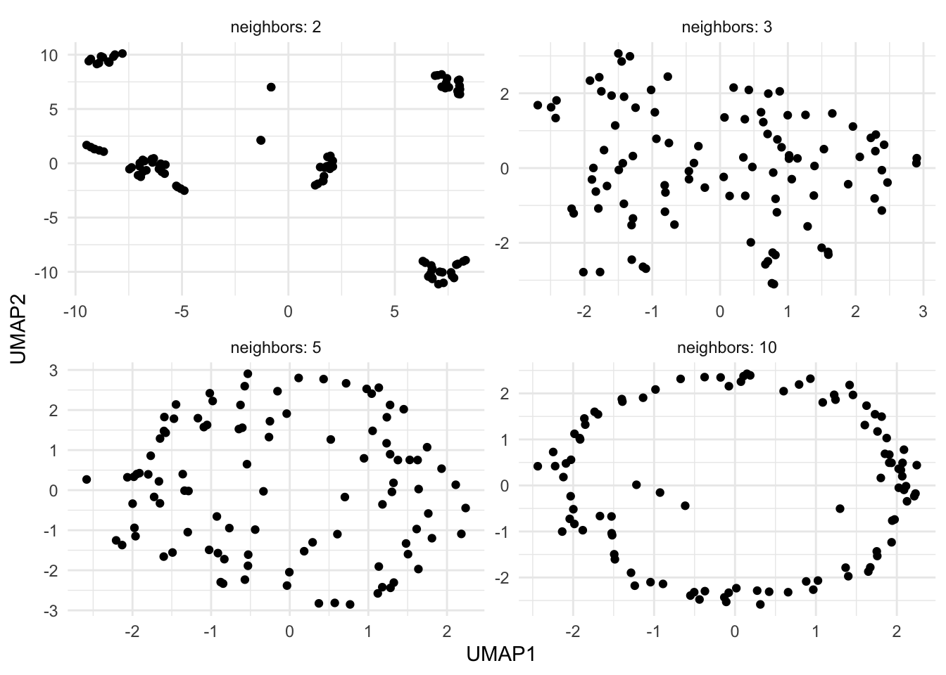
While UMAP is very popular, you need to be very careful when using it. The flexibility of UMAP is both its greatest strength and greatest weakness in feature engineering. Take a look at the figure below:
Warning: The `x` argument of `as_tibble.matrix()` must have unique column names if
`.name_repair` is omitted as of tibble 2.0.0.
ℹ Using compatibility `.name_repair`.
Here we have 4 different applications of UMAP with different values of n_neighbors. Depending on the value, we either see clusters, structure, or no structure at all. This figure used the exact same data in all 4 applications, with the original data being normally distributed.
You are discouraged from using small values of n_neighbors for similar reasons, but it is worth noting that you might fool yourself into finding relationships in your data that aren’t there. This is even more important for feature engineering, as it can be harder to visually validate the results in higher dimensions.
You use UMAP more to extract separation between clusters in the data, and to preserve local structure, than to generate components that in and of themselves contain valuable information. This is one of the reasons why UMAP is so popular in clustering projects.
76.2 Pros and Cons
76.2.1 Pros
Fairly fast
76.2.2 Cons
Very little explainability
Has a lot of hyperparameters
76.3 R Examples
We will be using the ames data set for these examples.