Warning: Using `size` aesthetic for lines was deprecated in ggplot2 3.4.0.
ℹ Please use `linewidth` instead.
ℹ The deprecated feature was likely used in the corrr package.
  Please report the issue at <https://github.com/tidymodels/corrr/issues>.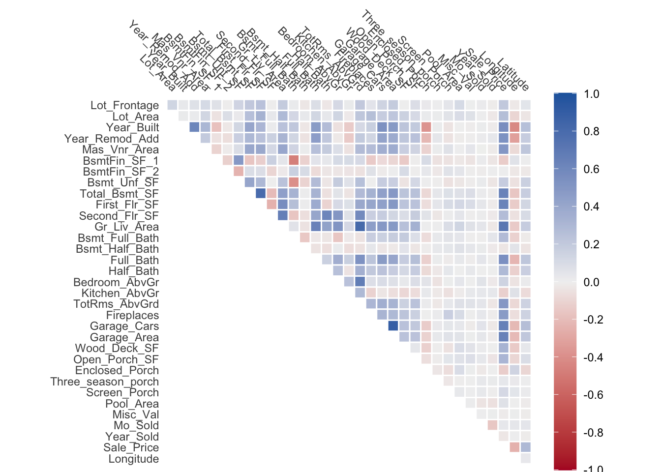
We are looking to remove correlated features. By correlated features, we typically talk about Pearson correlation. The methods in this chapter don’t require that Pearson correlation is used, just that any correlation method is used. Next, we will look at how we can remove the offending variables. We will show an iterative approach and a clustering approach. Both methods are learned methods as they identify variables to be kept.
I always find it useful to look at a correlation matrix first
Warning: Using `size` aesthetic for lines was deprecated in ggplot2 3.4.0.
ℹ Please use `linewidth` instead.
ℹ The deprecated feature was likely used in the corrr package.
Please report the issue at <https://github.com/tidymodels/corrr/issues>.looking at the above chart we see some correlated features. One way to perform our filtering is to find all the correlated pairs over a certain threshold and remove one of them. Below is a chart of the 10 most correlated pairs
| x | y | r |
|---|---|---|
| Garage_Cars | Garage_Area | 0.890 |
| Gr_Liv_Area | TotRms_AbvGrd | 0.808 |
| Total_Bsmt_SF | First_Flr_SF | 0.800 |
| Gr_Liv_Area | Sale_Price | 0.707 |
| Bedroom_AbvGr | TotRms_AbvGrd | 0.673 |
| Second_Flr_SF | Gr_Liv_Area | 0.655 |
| Garage_Cars | Sale_Price | 0.648 |
| Garage_Area | Sale_Price | 0.640 |
| Total_Bsmt_SF | Sale_Price | 0.633 |
| Gr_Liv_Area | Full_Bath | 0.630 |
One way to do filtering is to pick a threshold and repeatably remove one of the variables of the most correlated pair until there are no pairs left with a correlation over the threshold. This method has a minimal computational footprint as it just needs to calculate the correlations once at the beginning. The threshold is likely to need to be tuned as we can’t say for sure what a good threshold is. With the removal of variables, there is always a chance that we are removing signal rather than noise, this is increasingly true as we remove more and more predictors.
rewrite this as an algorithm
If we look at the above table, we notice that some of the variables occur together. One such example is Garage_Cars, Garage_Area and Sale_Price. These 3 variables are highly co-correlated and it would be neat if we could deal with these variables at the same time.
find a different example so Sale_Price isn’t part of this as it is usually the outcome.
Add a good graph showing this effect.
What we could do, is take the correlation matrix and apply a clustering model on it. Then we use the clustering model to lump together the groups of highly correlated predictors. Then within each cluster, one predictor is chosen to be kept. The clusters should ideally be chosen such that uncorrelated predictors are alone in their cluster. This method can work better with the global structure of the data but requires fitting and tuning another model.
We will use the ames data set from {modeldata} in this example. The {recipes} step step_corrr() performs the simple correlation filter described at the beginning of this chapter.
library(recipes)
library(modeldata)

corr_rec <- recipe(Sale_Price ~ ., data = ames) |>
  step_corr(all_numeric_predictors(), threshold = 0.75) |>
  prep()
We can see the variables that were removed with the tidy() method
corr_rec |>
  tidy(1)
# A tibble: 3 × 2
terms id
<chr> <chr>
1 First_Flr_SF corr_Bp5vK
2 Gr_Liv_Area corr_Bp5vK
3 Garage_Cars corr_Bp5vKWe can see that when we lower this threshold to the extreme, more predictors are removed.
recipe(Sale_Price ~ ., data = ames) |>
  step_corr(all_numeric_predictors(), threshold = 0.25) |>
  prep() |>
  tidy(1)
# A tibble: 13 × 2
terms id
<chr> <chr>
1 Bsmt_Unf_SF corr_RUieL
2 Total_Bsmt_SF corr_RUieL
3 First_Flr_SF corr_RUieL
4 Gr_Liv_Area corr_RUieL
5 Bsmt_Full_Bath corr_RUieL
6 Full_Bath corr_RUieL
7 TotRms_AbvGrd corr_RUieL
8 Fireplaces corr_RUieL
9 Garage_Cars corr_RUieL
10 Garage_Area corr_RUieL
11 Year_Built corr_RUieL
12 Second_Flr_SF corr_RUieL
13 Year_Remod_Add corr_RUieLI’m not aware of a good way to do this in a scikit-learn way. Please file an issue on github if you know of a good way.