43  Simple Imputation

43.1 Simple Imputation

When dealing with missing data, the first suggestion is often imputation. Simple imputation as covered in this chapter refers to the method where for each variable a single value is selected, and all missing values will be replaced by that value. It is important to remind ourselves why we impute missing values. Because the model we are using isn’t able to handle missing values natively. Simple imputation is the simplest way to handle missing values.

The way we find this value will depend on the variable type, and within each type of variable, we find multiple ways to decide on a value. The main categories are categorical and numeric variables.

For categorical we have 2 main options. We can replace the value of NA with "missing" or some other unused value. This would denote that the value was missing, without trying to pick a value. It would change the cardinality of the predictors as variables with levels “new”, “used”, and “old” would go from 3 levels to 4. Which may be undesirable. Especially with ordinal variables as it is unclear where the "missing" should go in the ordering.

The simple imputation way to deal with categorization is to find the value that we want to impute with. Typically this will be calculated with the mode, e.i. the most frequent value. It doesn’t have to be the most frequent value, you could set up the imputation to pick the 5th most common value or the least common value. But this is quite uncommon, and the mode is used by far the most. These methods also work for low cardinality integers.

For numeric values, we don’t have the option to add a new type of value. One option is to manually select the imputed value. If this approach is taken, then it should be done with utmost caution! It would also make it an unlearned imputation method. What is typically done is that some value is picked as the replacement. Be it the median, mean or even mode.

Datetime variables will be a different story. One could use the mode, or an adjusted mean or median. Another way is to let the value extraction work first, and then apply imputation to the extracted variables. Time series data is different enough that it has its chapter in Chapter 116.

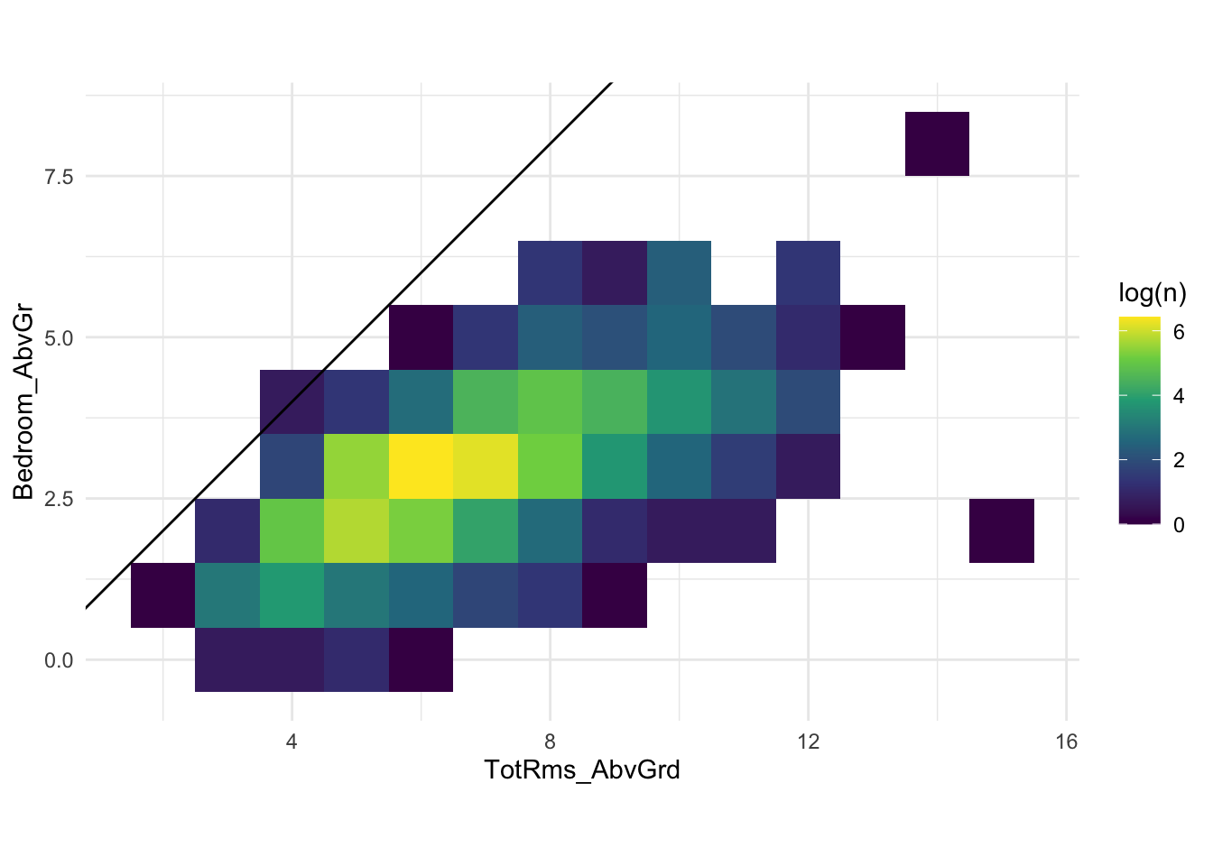
One of the main downsides to simple imputation is that it can lead to impossible configurations in the data. Imagine that the total square area is missing, but we know the number of rooms and number of bedrooms. Certain combinations are more likely than others. Below is the classic ames data set

Figure 43.1: All houses have fewer bedrooms than rooms themselves.

There can’t be more bedrooms than the total number of rooms. And we see that in the data. The average number of bedrooms is 2.85, and if we round, then it will be 3. That is perfectly fine for a house with an average number of rooms, but it will be impossible for small houses and quite inadequate for large houses. This is bad but can be seen as an improvement to the situation where the model didn’t fit because a missing value was present. This scenario is part of the motivation for Chapter 44.

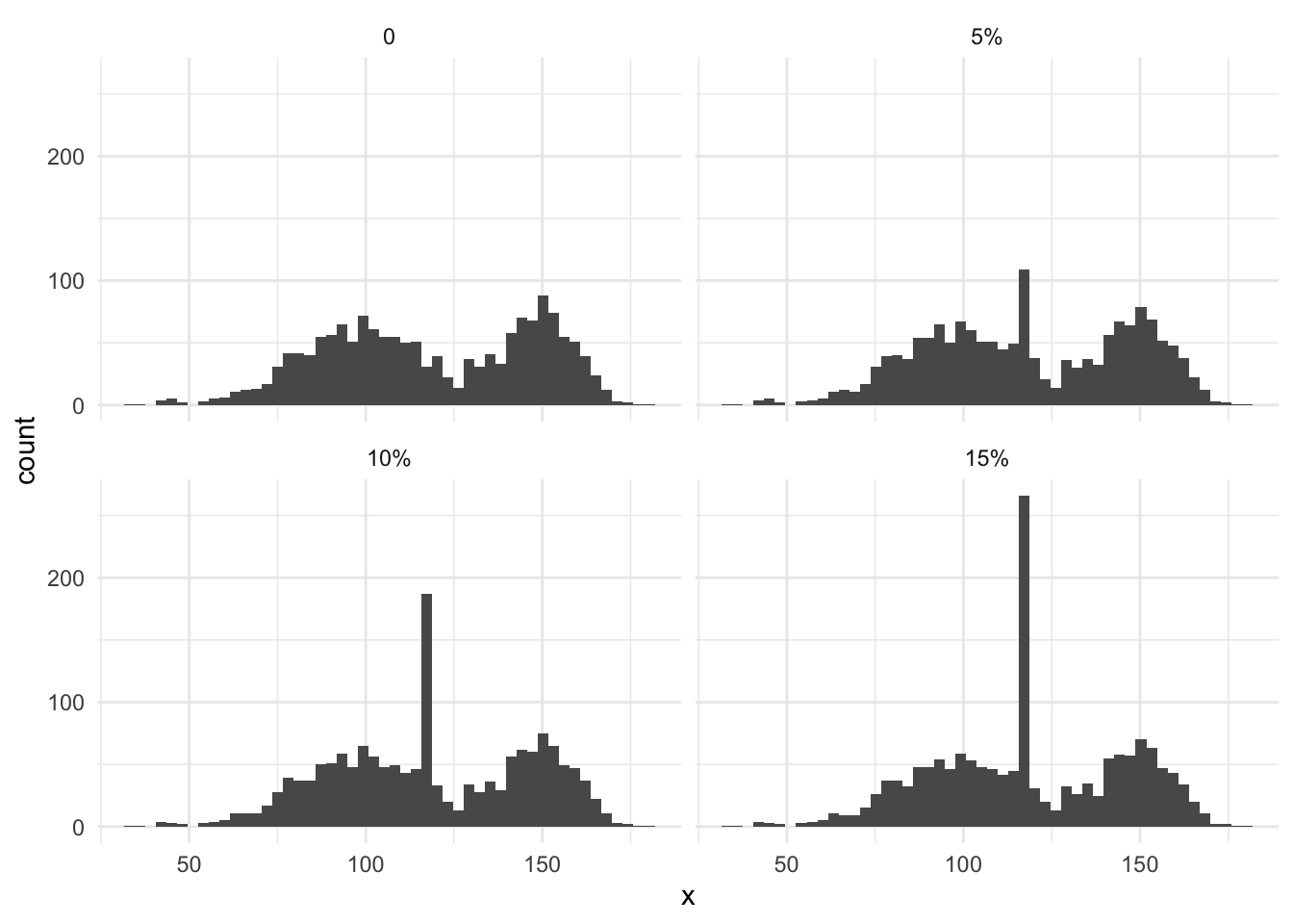
Other drawbacks of simple include; reducing the variance and standard deviation of the data. This happens because we are adding zero-variance information to the variables. In the same vein, we are changing the distribution of our variables, which can also affect downstream modeling and feature engineering.

Below we see this in effect, as more and more missing data, leads to a larger peak of the mean of the distribution.

Figure 43.2: Same distribution with a longer and longer spike at the mean.

Another thing we can do, while we stay in this domain of only using a single variable to impute itself, is to impute using the original distribution. So instead of imputing by the mode, a sample is drawn from the non-missing values, and that value is used. This is then done for each observation. Each observation won’t get the same values, but it will preserve the distribution, variance and standard deviation. It won’t help with the relationship between variables and as an added downside, it adds noise into imputation, making it a seeded feature engineering method.

On the implementation side, we need to be careful about how we extract the original distribution. This distribution needs to be saved for later reapply. Imagine a numeric predictor, if it is a non-integer, it will likely take many unique values, if not all unique values. We might want to bin the data to create a distribution that way to the same memory.

43.2 Pros and Cons

43.2.1 Pros

• Fast computationally
• Easy to explain what was done

43.2.2 Cons

• Doesn’t preserve relationship between predictors
• reducing the variance and standard deviation of the data
• unlikely to help performance

43.3 R Examples

The recipes package contains several steps. It includes the steps step_impute_mean(), step_impute_median() and step_impute_mode() which imputes by the mean, median and mode respectively.

TODO

find a good data set with missing values

library(recipes)
library(modeldata)

impute_rec <- recipe(Sale_Price ~ ., data = ames) |>
  step_impute_mean(contains("Area")) |>
  step_impute_median(contains("_SF")) |>
  step_impute_mode(all_nominal_predictors()) |>
  prep()

We can use the tidy() function to find the estimated mean

impute_rec |>
  tidy(1)

# A tibble: 5 × 3
  terms         value id               
  <chr>         <dbl> <chr>            
1 Lot_Area     10148  impute_mean_CnWw4
2 Mas_Vnr_Area   101. impute_mean_CnWw4
3 Gr_Liv_Area   1500  impute_mean_CnWw4
4 Garage_Area    473. impute_mean_CnWw4
5 Pool_Area        2  impute_mean_CnWw4

estimated median

impute_rec |>
  tidy(2)

# A tibble: 8 × 3
  terms         value id                 
  <chr>         <dbl> <chr>              
1 BsmtFin_SF_1     3  impute_median_UoO9a
2 BsmtFin_SF_2     0  impute_median_UoO9a
3 Bsmt_Unf_SF    466. impute_median_UoO9a
4 Total_Bsmt_SF  990  impute_median_UoO9a
5 First_Flr_SF  1084  impute_median_UoO9a
6 Second_Flr_SF    0  impute_median_UoO9a
7 Wood_Deck_SF     0  impute_median_UoO9a
8 Open_Porch_SF   27  impute_median_UoO9a

and estimated mode

impute_rec |>
  tidy(3)

# A tibble: 40 × 3
   terms        value                               id               
   <chr>        <chr>                               <chr>            
 1 MS_SubClass  One_Story_1946_and_Newer_All_Styles impute_mode_I3pVC
 2 MS_Zoning    Residential_Low_Density             impute_mode_I3pVC
 3 Street       Pave                                impute_mode_I3pVC
 4 Alley        No_Alley_Access                     impute_mode_I3pVC
 5 Lot_Shape    Regular                             impute_mode_I3pVC
 6 Land_Contour Lvl                                 impute_mode_I3pVC
 7 Utilities    AllPub                              impute_mode_I3pVC
 8 Lot_Config   Inside                              impute_mode_I3pVC
 9 Land_Slope   Gtl                                 impute_mode_I3pVC
10 Neighborhood North_Ames                          impute_mode_I3pVC
# ℹ 30 more rows

TODO

wait for the distribution step

43.4 Python Examples

We are using the ames data set for examples. {sklearn} provided the SimpleImputer() method we can use. The main argument we will use is strategy which we can set to determine the type of imputing.

from feazdata import ames
from sklearn.compose import ColumnTransformer
from sklearn.impute import SimpleImputer

ct = ColumnTransformer(
    [('mean_impute', SimpleImputer(strategy='mean'), ['Sale_Price', 'Lot_Area', 'Wood_Deck_SF',  'Mas_Vnr_Area'])], 
    remainder="passthrough")

ct.fit(ames)

ColumnTransformer(remainder='passthrough',
                  transformers=[('mean_impute', SimpleImputer(),
                                 ['Sale_Price', 'Lot_Area', 'Wood_Deck_SF',
                                  'Mas_Vnr_Area'])])

In a Jupyter environment, please rerun this cell to show the HTML representation or trust the notebook.
On GitHub, the HTML representation is unable to render, please try loading this page with nbviewer.org.

ct.transform(ames)

      mean_impute__Sale_Price  ...  remainder__Latitude
0                    215000.0  ...               42.054
1                    105000.0  ...               42.053
2                    172000.0  ...               42.053
3                    244000.0  ...               42.051
4                    189900.0  ...               42.061
...                       ...  ...                  ...
2925                 142500.0  ...               41.989
2926                 131000.0  ...               41.988
2927                 132000.0  ...               41.987
2928                 170000.0  ...               41.991
2929                 188000.0  ...               41.989

[2930 rows x 74 columns]

Setting strategy='median' switches the imputer to do median imputing.

ct = ColumnTransformer(
    [('median_impute', SimpleImputer(strategy='median'), ['Sale_Price', 'Lot_Area', 'Wood_Deck_SF',  'Mas_Vnr_Area'])], 
    remainder="passthrough")

ct.fit(ames)

ColumnTransformer(remainder='passthrough',
                  transformers=[('median_impute',
                                 SimpleImputer(strategy='median'),
                                 ['Sale_Price', 'Lot_Area', 'Wood_Deck_SF',
                                  'Mas_Vnr_Area'])])

In a Jupyter environment, please rerun this cell to show the HTML representation or trust the notebook.
On GitHub, the HTML representation is unable to render, please try loading this page with nbviewer.org.

ct.transform(ames)

      median_impute__Sale_Price  ...  remainder__Latitude
0                      215000.0  ...               42.054
1                      105000.0  ...               42.053
2                      172000.0  ...               42.053
3                      244000.0  ...               42.051
4                      189900.0  ...               42.061
...                         ...  ...                  ...
2925                   142500.0  ...               41.989
2926                   131000.0  ...               41.988
2927                   132000.0  ...               41.987
2928                   170000.0  ...               41.991
2929                   188000.0  ...               41.989

[2930 rows x 74 columns]