94 Edited Nearest Neighbor
94.1 Edited Nearest Neighbor
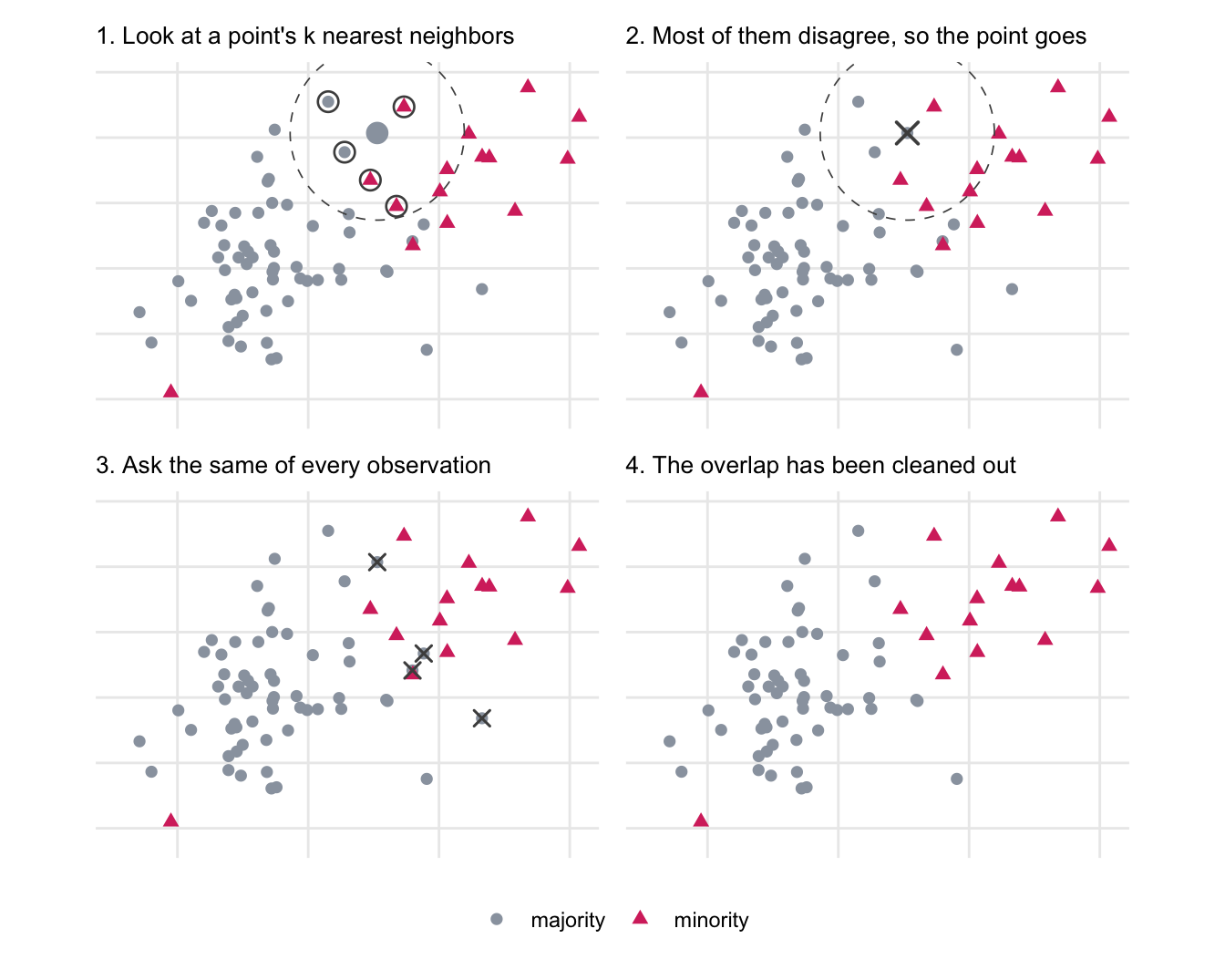
This method is another undersampling method, it works by removing observations close to the decision boundary between classes (Wilson 1972). This method tries to remove observations that would otherwise be hard to classify.
The algorithm goes as follows:
- Compute the k nearest neighbors for each observation in the data set.
- Remove observations from the majority class if the removal criteria are satisfied.
The removal criteria is something we can choose different options for. A typical implementation will either remove an observation if the majority of the neighbors are of a different class, but you could also tighten this and remove an observation if any of the neighbors are of a different class.
Figure 94.1 works through the majority-vote criterion one point at a time.
The idea is that we are able to remove noisy observations this way. And depending on which criteria you choose, you could see how that would be. By only allowing us to keep all the observations that have neighbors all of the same class, we can end up removing a lot of the decision boundary, especially any area where there is overlap.
The general framework is described in terms of 2 classes, but it extends to more without any reduction, and so is one of the methods in Section 86.2 that needs no expanding. Both removal criteria are phrased as comparisons against the observation’s own label: the “any” criterion asks whether any neighbor carries a different label, and the majority-vote criterion compares the observation’s label against the most common label among its neighbors. Neither question needs the other classes pooled together, and both look at the true labels throughout.
It does still change how things play out. In the two-class case, any majority point deeply embedded in the minority class will most likely be removed. With three or more classes, a single observation from one majority class deeply embedded in another majority class will not only be deleted itself, but will take its neighbors with it if we use the “any” criterion. This feels less ideal and is something we have to think about when applying this method.
By itself, this method is simple, and there have been a couple of method that expands on the foundation of this method. The first one is Repeated Edited Nearest Neighbor (Tomek 1976). And it does what it says, it repeats Edited Nearest Neighbor a number of times. You can either set it up such that it runs a fixed number of times or until no observations are removed during an iteration.
Another named variant AllKNN. This is a variant of Edited Nearest Neighbors, where you select a value of k, then apply ENN with neighbors 1 through k. Both of these variants result in more observations being removed.
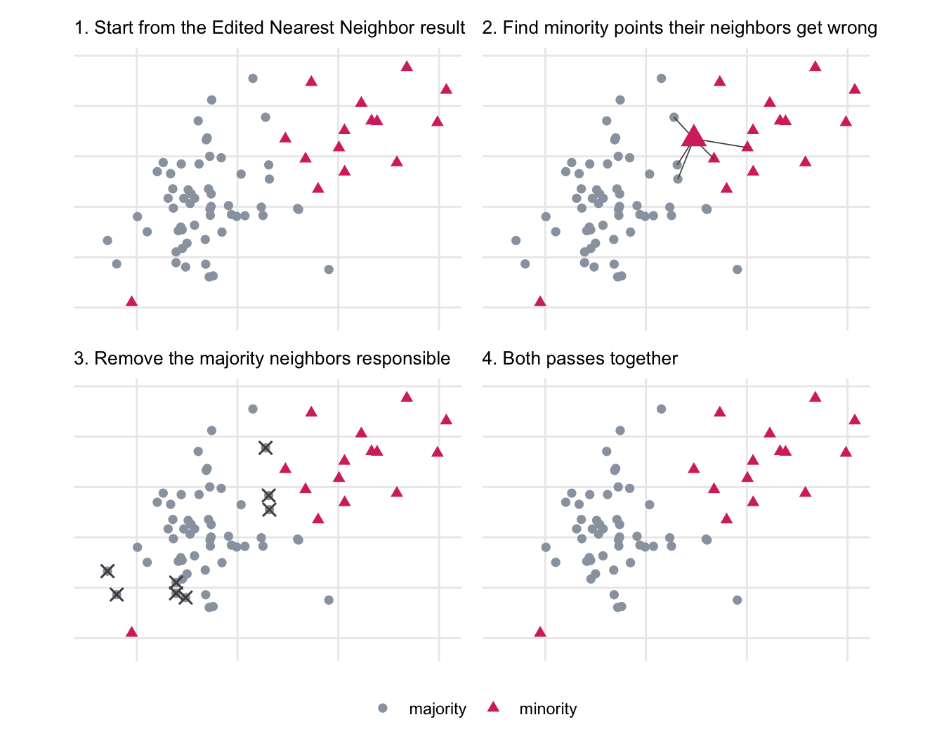
The last extension we will talk about is the Neighborhood Cleaning Rule (Laurikkala 2001). This method starts by running Edited Nearest Neighbor. Then we run a K Nearest Neighbors on the minority observations. Any majority class observations that misclassify a minority observation will be removed as well. Note that this second stage does not inherit the multi-class behavior of the first: it needs to designate one class as “the minority”, and the usual choice is the single smallest class, with the remaining classes acting as a pooled majority. That makes this half of the method the single-application strategy from Section 86.2 rather than a true one-vs-rest. Implementations typically also skip cleaning around classes that are themselves small relative to the smallest one. Figure 94.2 shows the second pass, which is where the two methods part ways.
Like all the methods in this section, this changes the distribution of the training data set, which is covered in Section 86.3.
TipAnimated version
The same walkthroughs, one step at a time, are available as animated slides for Edited Nearest Neighbor and the Neighborhood Cleaning Rule.
94.2 Pros and Cons
94.2.1 Pros
94.2.2 Cons
94.3 R Examples
We will be using the same subset of the ames data set as in the up-sampling chapter.
library(recipes)
library(themis)
library(modeldata)
library(dplyr)
data("ames")

ames_imbalance <- ames |>
  filter(MS_Zoning %in% c("Residential_Low_Density", "Residential_Medium_Density")) |>
  mutate(MS_Zoning = droplevels(MS_Zoning)) |>
  select(MS_Zoning, Lot_Area, Year_Built, Gr_Liv_Area, Full_Bath)

ames_imbalance |>
  count(MS_Zoning)
# A tibble: 2 × 2
MS_Zoning n
<fct> <int>
1 Residential_Low_Density 2273
2 Residential_Medium_Density 462{themis} provides step_enn(). All three of the variants described above are reachable from this one step.
The times argument gives Repeated Edited Nearest Neighbors.
recipe(MS_Zoning ~ ., data = ames_imbalance) |>
  step_enn(MS_Zoning, times = 3) |>
  prep() |>
  bake(new_data = NULL) |>
  count(MS_Zoning)
# A tibble: 2 × 2
MS_Zoning n
<fct> <int>
1 Residential_Low_Density 2176
2 Residential_Medium_Density 225And all_k gives AllKNN.
recipe(MS_Zoning ~ ., data = ames_imbalance) |>
  step_enn(MS_Zoning, all_k = TRUE) |>
  prep() |>
  bake(new_data = NULL) |>
  count(MS_Zoning)
# A tibble: 2 × 2
MS_Zoning n
<fct> <int>
1 Residential_Low_Density 2094
2 Residential_Medium_Density 214The Neighborhood Cleaning Rule is a separate step, step_ncl().
recipe(MS_Zoning ~ ., data = ames_imbalance) |>
  step_ncl(MS_Zoning) |>
  prep() |>
  bake(new_data = NULL) |>
  count(MS_Zoning)
# A tibble: 2 × 2
MS_Zoning n
<fct> <int>
1 Residential_Low_Density 1757
2 Residential_Medium_Density 462