89 SMOTE Variants

89.1 SMOTE Variants

While SMOTE provides the basis of the method, it is often not good enough by itself, as it has a long list of issues and constraints. Each of these variants builds on the base SMOTE algorithm by changing or adding parts of it to handle a specific use case.

89.1.1 Non-numeric variants

The first constraint that is often found with SMOTE is that you are limited to using numeric predictors. The SMOTEN and SMOTENC try to handle this in two different ways. Both were introduced alongside the original SMOTE method (Chawla et al. 2002). Synthetic minority oversampling technique for Nominal (SMOTEN) is a modification of SMOTE that works with categorical data. Since the method is focused on categorical input we can’t use the traditional nearest neighbor, instead we use the Value Difference Metric (VDM) as a way to calculate categorical distances. Where SMOTE samples random points on the line between points and their neighbor, SMOTEN calculates the most frequent category for each feature between the pair of points.

The obvious biggest constraint with this method is that it requires all the predictors to be categorical. Arguably even more rare than having all numeric predictors.

While each predictor is able to generate invalid values, as they are taken directly from the training data. We are not guaranteed that the combinations of the most frequent level within each predictor combines to a plausible observation.

Another variant Synthetic Minority Over-sampling Technique for Nominal and Continuous (SMOTENC) tries to combine SMOTE and SMOTEN. A combined distance metric is used to calculate neighbors and numeric predictors are generated using the SMOTE method. And categorical predictors are generated with the SMOTEN way.

89.1.2 Boundary-focused variants

The original SMOTE method generated new synthetic samples from all the observations within the class. The worry is that this will generate a lot of points in the “safe” areas of the distribution where they aren’t as useful. Instead, we should generate observations near the border of the distribution of the class itself, as those are the observations that actually matter for our decision boundaries. This idea is known as Borderline-SMOTE (Han et al. 2005).

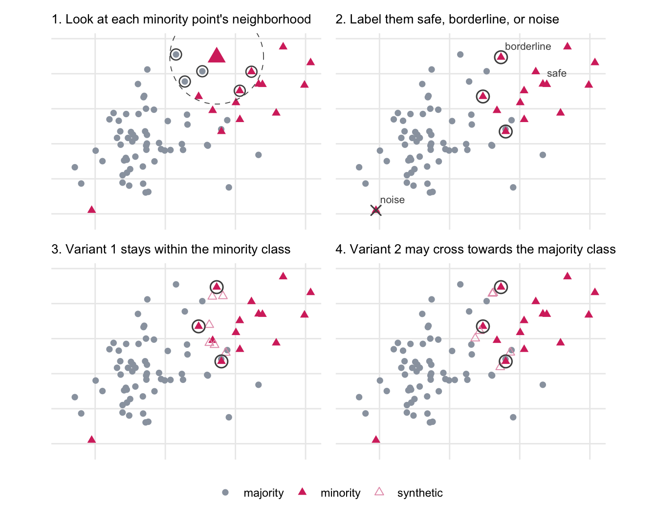
To determine whether an observation is considered borderline or not, we calculate the nearest neighbors of each observation in the data set. And we look to see whether the neighbors are of the same class or not. If all the neighbors of an observation are of different classes, then the observation is labeled as “noise”. Likewise, if too many of the neighbors of an observation are of the same class as itself, the observation is labeled “safe” otherwise, it is labeled “borderline”. The threshold of too many is typically 50%.

We will generate new synthetic observations around the neighbors of all the borderline observations. And we have two major ways to do it. Either we do it like we did in standard SMOTE where we generate points between an observation and neighbors of the same class, or we could generate points between any of the neighbors, regardless of whether they are of the same class or not. This is referred to as variants 1 and 2, respectively.

Variant 1 is more aggressive, as it produces points closer to the decision boundary, And the choice to label fully enclosed points as noise is a way to avoid having issues here.

Figure 89.1 shows both the labeling step and the difference between the two variants.

Four scatter plots in a 2x2 grid showing a gray majority class and a pink minority class meeting along a diagonal. Panel 1: one minority point near the boundary has a dashed circle around it enclosing its five nearest neighbors, a mix of gray and pink. Panel 2: minority points are labeled, with dark rings on the borderline points along the diagonal, a cross on the lone noise point stranded in the majority cloud, and nothing on the safe points deep in the minority region. Panel 3: hollow synthetic points appear only around the ringed borderline points, all on the minority side. Panel 4: the same, except some synthetic points now sit on the majority side of the boundary. — Figure 89.1: Borderline-SMOTE first sorts the minority observations into safe, borderline, and noise, then generates only around the borderline ones. Variant 2 is allowed to interpolate towards the majority class.

89.1.3 Distribution

Borderline SMOTE, as seen before, focused on sampling observations near the border. Having a hard rule to decide which observation should be included. Adaptive Synthetic Sampling (ADASYN) asks a different question (He et al. 2008).

Each observation is given a score based on how many neighbours it shares with the majority class. Instead of generating a threshold based on this score, we instead use the score to sample which observations should be generated around.

This means that we try to generate observations around observations that are “harder” to classify. This is in contrast to borderline SMOTE, where all borderline points were treated the same.

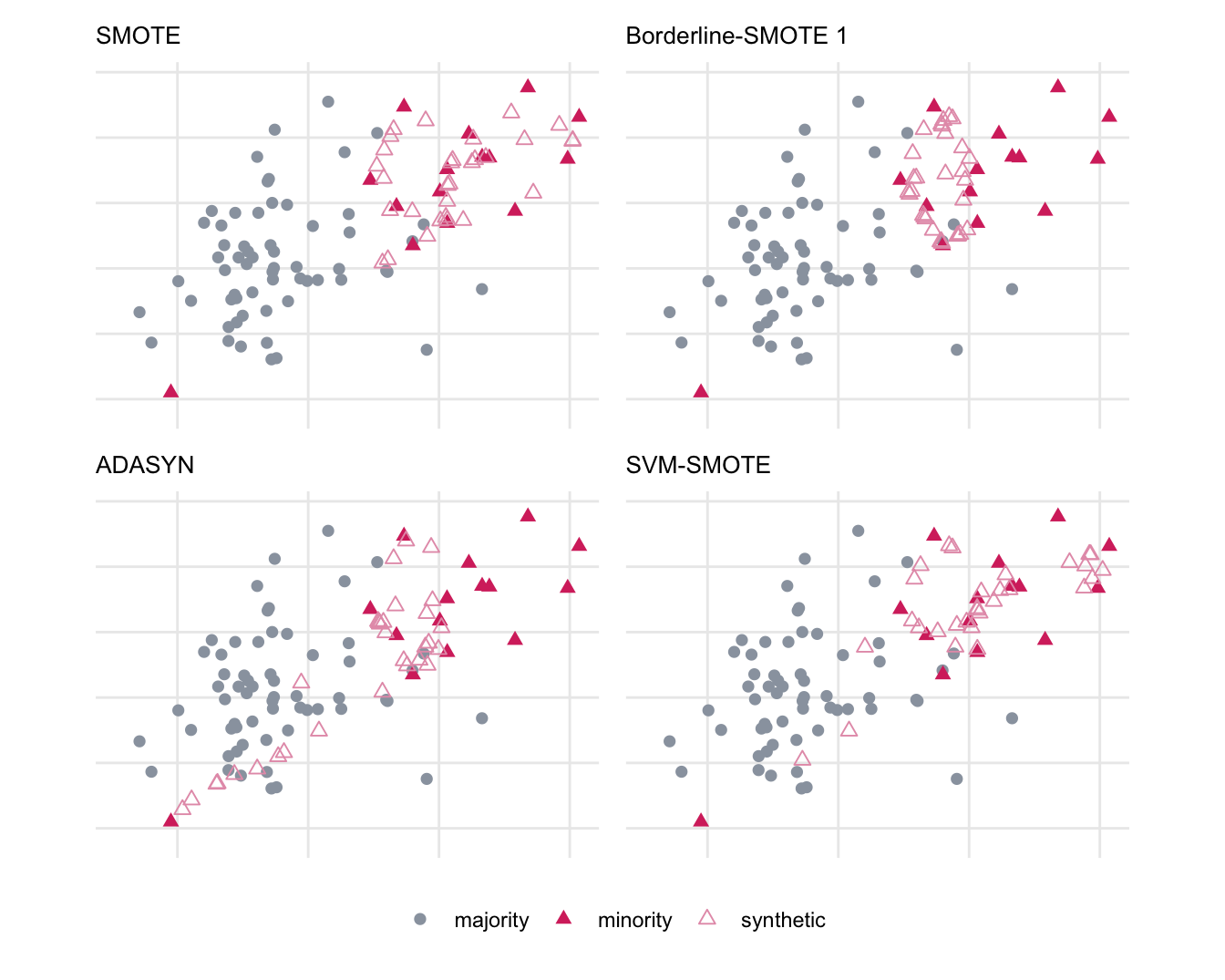
One of the downsides of this method is that there is no explicit exclusion to noisy observations. So a point from one class that is located entirely inside another class will still generate observations. It will in fact be one of the most attractive points to generate around, since every one of its neighbors belongs to the other class. You can see this in Figure 89.2 further down, where ADASYN lays a trail of synthetic observations between the lone outlier and the rest of its class.

89.1.4 Model-based

A different way to calculate the border is based on the idea of SVM. Instead of calculating the nearest neighbors to find borders, we fit an SVM model. Then we identify the support vectors from the minority classes, and finally generate synthetic observations around those support vectors. This method is typically called SVM SMOTE (Nguyen et al. 2011).

The three boundary-aware variants and base SMOTE all generate the same number of observations. What separates them is where those observations end up, which is what Figure 89.2 compares.

Four scatter plots in a 2x2 grid, each showing the same gray majority class and pink minority class with thirty hollow synthetic points added. In the SMOTE panel the synthetic points are spread evenly through the minority region. In the Borderline-SMOTE panel they sit in a tight band along the edge of the minority class facing the majority class. In the ADASYN panel they favor that same edge but a visible trail of them also runs down into the majority cloud towards the isolated minority point in the lower left. In the SVM-SMOTE panel they follow the boundary in a looser band that reaches further along it. — Figure 89.2: The same number of synthetic observations, placed by four different variants. Base SMOTE spreads them over the whole minority class, the others concentrate them near the boundary, and ADASYN also pours them along the path to the lone outlier.

89.1.5 Distance/Neighborhood-based variants

Another style of variant is one that changes the way you calculate neighbors. Typically, you use a nearest neighbor method based on Euclidean distances. However, Euclidean distances aren’t the only way to calculate distances between two points. This has led to a number of SMOTE variants purely based on using a different distance metric.

SMOTE-Cosine: Cosine distance
SMOTE-Mahalanobis: Mahalanobis distance
SMOTE-Manhattan: Manhattan distance
SMOTE-chebyshev: Chebyshev distance

89.1.6 Dimensionality reduction methods

This section and the next section both contain methods that we don’t consider real methods in this book. Instead they are multiple methods chained together one after another. This might have been done for performance reasons or as an implementation detail. But we think it is important that we treat each method as a building block that you can then combine to fully tackle your problem.

For the dimensionality reduction method, some of the common SMOTE “variants” include:

KMeansSMOTE: K-Means Clustering -> SMOTE
PCA SMOTE: PCA -> SMOTE
LDA SMOTE: LDA -> SMOTE

89.1.7 Chained methods

There are also a number of named SMOTE variants that are just SMOTE followed by another method commonly used with imbalanced data:

SMOTEENN: SMOTE -> Edited Nearest Neighbors
SMOTETomek: SMOTE -> Tomek Link removal
SMOTE-RSB: SMOTE -> Rough set boundary cleaning

89.1.8 Behavior with more than two classes

The variants described above do not all handle multiple classes the same way, and the split follows the strategies in Section 86.2.

SMOTEN and SMOTENC inherit base SMOTE’s behavior.

Borderline-SMOTE and ADASYN both need to know how many of an observation’s neighbors belong to a different class, which means they need a notion of “the other class.” Both resolve this with one-vs-rest.

Like all the methods in this section, these change the distribution of the training data set, which is covered in Section 86.3.

Animated versions

Several of these variants have animated walkthroughs: Borderline-SMOTE 1, Borderline-SMOTE 2, ADASYN, SVM-SMOTE, and k-means SMOTE.

89.2 R Examples

We will be using the same subset of the ames data set as in the up-sampling chapter. The categorical variants need their own data, so we set up two more versions of it at the same time.

library(recipes)
library(themis)
library(modeldata)
library(dplyr)
data("ames")

ames_base <- ames |>
  filter(MS_Zoning %in% c("Residential_Low_Density", "Residential_Medium_Density")) |>
  mutate(MS_Zoning = droplevels(MS_Zoning))

ames_imbalance <- ames_base |>
  select(MS_Zoning, Lot_Area, Year_Built, Gr_Liv_Area, Full_Bath)

ames_nominal <- ames_base |>
  select(MS_Zoning, Lot_Config, Bldg_Type, Heating_QC)

ames_mixed <- ames_base |>
  select(MS_Zoning, Lot_Area, Year_Built, Lot_Config, Bldg_Type)

ames_imbalance |>
  count(MS_Zoning)

# A tibble: 2 × 2
  MS_Zoning                      n
  <fct>                      <int>
1 Residential_Low_Density     2273
2 Residential_Medium_Density   462

step_smoten() handles the all-categorical case.

recipe(MS_Zoning ~ ., data = ames_nominal) |>
  step_smoten(MS_Zoning) |>
  prep() |>
  bake(new_data = NULL) |>
  count(MS_Zoning)

# A tibble: 2 × 2
  MS_Zoning                      n
  <fct>                      <int>
1 Residential_Low_Density     2273
2 Residential_Medium_Density  2273

step_smotenc() handles the mixed case, and works out which predictors are categorical on its own.

recipe(MS_Zoning ~ ., data = ames_mixed) |>
  step_smotenc(MS_Zoning) |>
  prep() |>
  bake(new_data = NULL) |>
  count(MS_Zoning)

# A tibble: 2 × 2
  MS_Zoning                      n
  <fct>                      <int>
1 Residential_Low_Density     2273
2 Residential_Medium_Density  2273

step_bsmote() is Borderline-SMOTE, and the all_neighbors argument selects between the two variants described above. FALSE gives variant 1, which only interpolates towards neighbors of the same class, and TRUE gives the more aggressive variant 2.

recipe(MS_Zoning ~ ., data = ames_imbalance) |>
  step_bsmote(MS_Zoning, all_neighbors = FALSE) |>
  prep() |>
  bake(new_data = NULL) |>
  count(MS_Zoning)

# A tibble: 2 × 2
  MS_Zoning                      n
  <fct>                      <int>
1 Residential_Low_Density     2273
2 Residential_Medium_Density  2273

recipe(MS_Zoning ~ ., data = ames_imbalance) |>
  step_bsmote(MS_Zoning, all_neighbors = TRUE) |>
  prep() |>
  bake(new_data = NULL) |>
  count(MS_Zoning)

# A tibble: 2 × 2
  MS_Zoning                      n
  <fct>                      <int>
1 Residential_Low_Density     2273
2 Residential_Medium_Density  2273

step_adasyn() is Adaptive Synthetic Sampling.

recipe(MS_Zoning ~ ., data = ames_imbalance) |>
  step_adasyn(MS_Zoning) |>
  prep() |>
  bake(new_data = NULL) |>
  count(MS_Zoning)

# A tibble: 2 × 2
  MS_Zoning                      n
  <fct>                      <int>
1 Residential_Low_Density     2273
2 Residential_Medium_Density  2273

step_svmsmote() is the SVM-based variant.

recipe(MS_Zoning ~ ., data = ames_imbalance) |>
  step_svmsmote(MS_Zoning) |>
  prep() |>
  bake(new_data = NULL) |>
  count(MS_Zoning)

# A tibble: 2 × 2
  MS_Zoning                      n
  <fct>                      <int>
1 Residential_Low_Density     2273
2 Residential_Medium_Density  2273

{themis} also provides step_kmeans_smote().

recipe(MS_Zoning ~ ., data = ames_imbalance) |>
  step_kmeans_smote(MS_Zoning) |>
  prep() |>
  bake(new_data = NULL) |>
  count(MS_Zoning)

# A tibble: 2 × 2
  MS_Zoning                      n
  <fct>                      <int>
1 Residential_Low_Density     2273
2 Residential_Medium_Density  2273

The distance-based variants listed above do not need separate steps. They are step_smote() with a different distance argument.