95 Instance Hardness Threshold
95.1 Instance Hardness Threshold
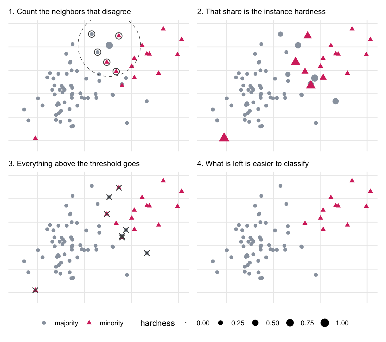
The Instance Hardness Threshold method is based on the notion of instance hardness (Smith et al. 2014). The general idea behind this method is that we operate under an assumption that each observation has a value associated with it, that signals how hard it is to classify correctly. Then removing the hard-to-classify observation, thereby giving the model an easier data set to work with [SMGC14].
We are essentially fitting an additional model, only letting through observations that this new model was able to work with easily. How exactly this is done in practice will depend on the implementation. Since each observation is given a value, typically the probability estimate of the model, we can remove how many or how few observations we want by setting a threshold. We can either remove a specific number of observations, a proportion of the data, or anything below a certain threshold value. Using the threshold value is somewhat tricky as it assumes that the model that we used is properly calibrated.
Some implementations allow for any classification model to be used, while other implementations pick a predefined method. Figure 95.1 uses the simplest of the predefined options, the k-Disagreeing Neighbors measure, where an observation’s hardness is the share of its neighbors that carry a different label.
This is the one method in this section that never had a two-class assumption to escape, and it needs no expanding in the sense of Section 86.2.
Like all the methods in this section, this changes the distribution of the training data set, which is covered in Section 86.3.
TipAnimated version
The same walkthrough, one step at a time, is available as an animated slide.
95.2 Pros and Cons
95.2.1 Pros
95.2.2 Cons
- The choice of model matters
- Potentially long fitting time depending on model choice
95.3 R Examples
We will be using the same subset of the ames data set as in the up-sampling chapter.
library(recipes)
library(themis)
library(modeldata)
library(dplyr)
data("ames")

ames_imbalance <- ames |>
  filter(MS_Zoning %in% c("Residential_Low_Density", "Residential_Medium_Density")) |>
  mutate(MS_Zoning = droplevels(MS_Zoning)) |>
  select(MS_Zoning, Lot_Area, Year_Built, Gr_Liv_Area, Full_Bath)

ames_imbalance |>
  count(MS_Zoning)
# A tibble: 2 × 2
MS_Zoning n
<fct> <int>
1 Residential_Low_Density 2273
2 Residential_Medium_Density 462{themis} provides step_instance_hardness(). This is the neighborhood-based version described above, using the k-Disagreeing Neighbors measure, so there is no model to specify.
recipe(MS_Zoning ~ ., data = ames_imbalance) |>
  step_instance_hardness(MS_Zoning) |>
  prep() |>
  bake(new_data = NULL) |>
  count(MS_Zoning)
# A tibble: 2 × 2
MS_Zoning n
<fct> <int>
1 Residential_Low_Density 462
2 Residential_Medium_Density 462