91 Near-Miss
91.1 Near-Miss
The NearMiss method is a method that is used to remove observations from the majority classes (Mani and Zhang 2003). Like with many of the other methods in this section, we are going to focus on points based on their distance to instances of other classes.
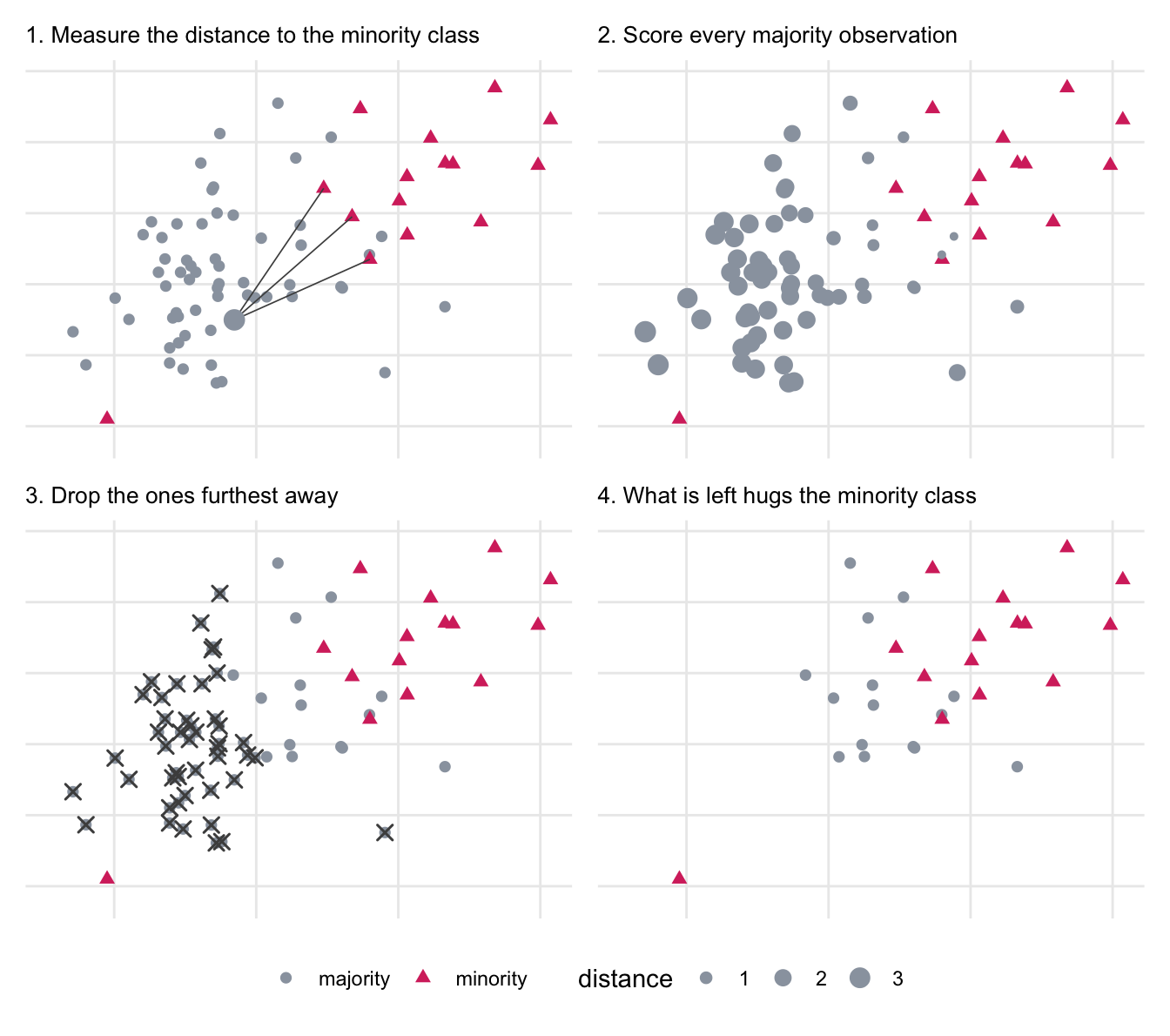
What we are doing is that we are removing points from the majority class that are far away from the minority class. We are keeping points from the majority class that are close to the minority class. In other words, we are only keeping the “near misses”. While the idea is fairly straightforward, it has 3 different recognized variants based on how we define a near miss.
- NearMiss-1: Selects majority class observations with the smallest average distance to the three closest minority class observations.
- NearMiss-2: Selects majority class observations with the smallest average distance to the three furthest minority class observations.
- NearMiss-3: It is a two-stage method, first for each minority class, their nearest neighbors are kept, and then we select the majority class observations with the smallest distance to each minority class observation.
While the distinction between the 1 and 2 variants might seem small, what you are getting is that with NearMiss-1, you are preserving samples that are most similar to the minority class, and with NearMiss-2, you are preserving samples that are least similar to the minority class. NearMiss-3 is trying to have a more blended selection.
This method, like many of the other methods, is technically not restricted to be used on the majority class, and could, in theory, be used on any number of classes in the data set.
Doing so requires settling a question the original description leaves open. All three variants are defined by distances from majority observations to the minority class, which is unambiguous only when there are two classes. NearMiss resolves this with the one-vs-rest strategy from Section 86.2.
Figure 91.1 walks through NearMiss-1, which is the most direct of the three.
One of the convenient things about this method is that it technically works by giving the observations an ordering, And we just have to find the cut point that determines how many points to retain.
Like all the methods in this section, this changes the distribution of the training data set, which is covered in Section 86.3.
TipAnimated version
The same walkthrough, one step at a time, is available as an animated slide.
91.2 Pros and Cons
91.2.1 Pros
91.2.2 Cons
91.3 R Examples
We will be using the same subset of the ames data set as in the up-sampling chapter.
library(recipes)
library(themis)
library(modeldata)
library(dplyr)
data("ames")

ames_imbalance <- ames |>
  filter(MS_Zoning %in% c("Residential_Low_Density", "Residential_Medium_Density")) |>
  mutate(MS_Zoning = droplevels(MS_Zoning)) |>
  select(MS_Zoning, Lot_Area, Year_Built, Gr_Liv_Area, Full_Bath)

ames_imbalance |>
  count(MS_Zoning)
# A tibble: 2 × 2
MS_Zoning n
<fct> <int>
1 Residential_Low_Density 2273
2 Residential_Medium_Density 462{themis} provides step_nearmiss(), and the version argument selects which of the three variants to use.
recipe(MS_Zoning ~ ., data = ames_imbalance) |>
  step_nearmiss(MS_Zoning, version = 1) |>
  prep() |>
  bake(new_data = NULL) |>
  count(MS_Zoning)
# A tibble: 2 × 2
MS_Zoning n
<fct> <int>
1 Residential_Low_Density 462
2 Residential_Medium_Density 462