88 SMOTE
88.1 SMOTE
The goal of the Synthetic minority oversampling technique (SMOTE) is to deal with imbalanced data using synthetically generated samples (Chawla et al. 2002).
this method is in a way similar to up-sampling, But there is a twist. Instead of sampling observations from the minority classes, We instead generate new observations based on the characteristics of the data set.
Generally works for categorical outcomes (hence imbalance), and the base case only works with numeric data with no missingness.
We start by identifying the minority classes and the majority class. counting how many observations are in each, as this will be used as a target for how many observations to generate.
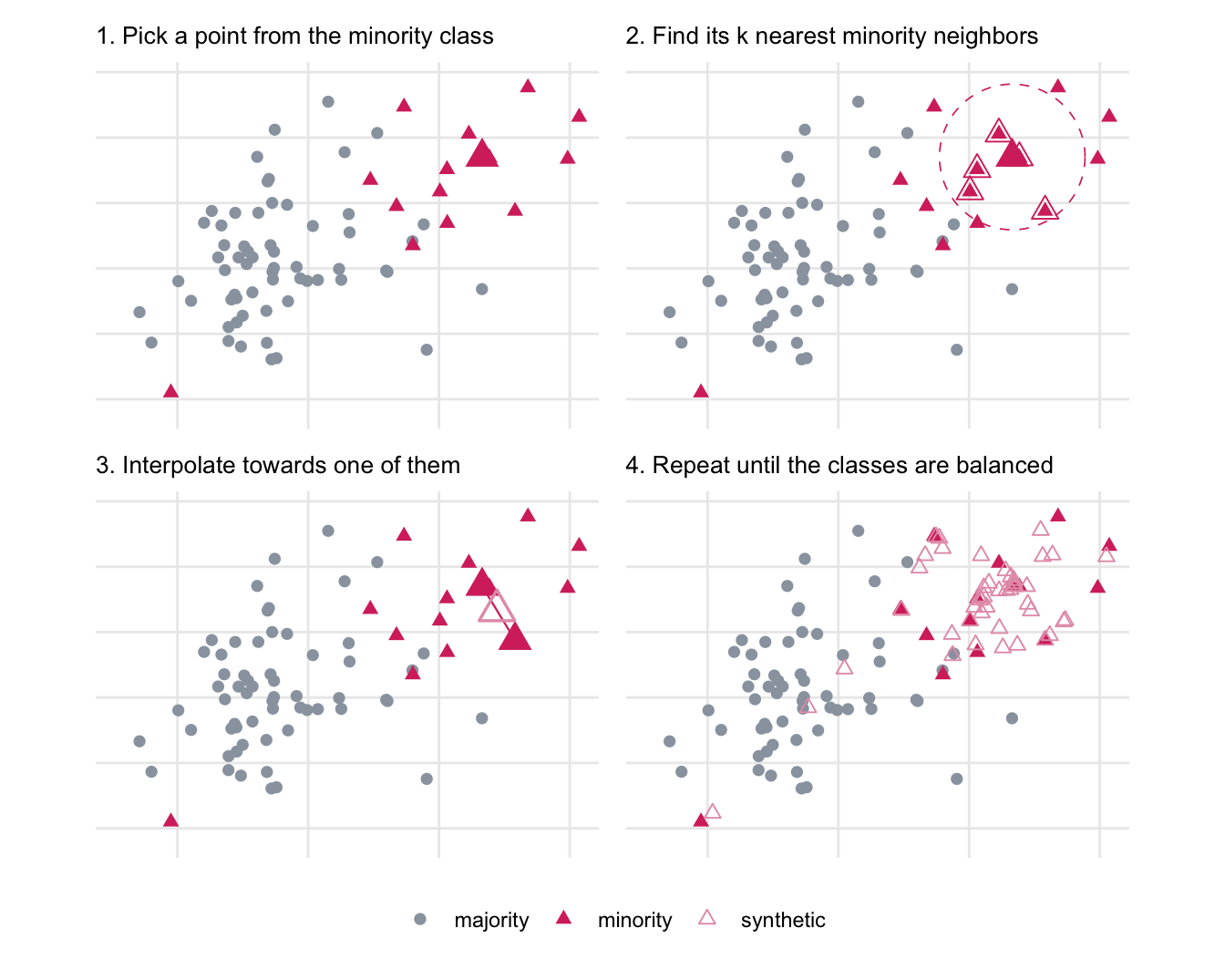
Between each minority class, you calculate all the nearest neighbors. Then, for each observation, you are randomly picking one of its close neighbors (typically k= 5) as its designated neighbor for the task. Then a synthetic observation is generated at random on the line between these two points. This is typically done for every observation. With multiple runs, depending on how many observations will need to be created. A different random neighbor is picked each time, as well as a random point on the spanning line.
You generally have a ratio threshold, determining how many observations you need. If you want a precise match for the counts of observations, you can randomly select observations to generate during the last run for a precise number of generated observations.
Figure 88.1 walks through the whole procedure on a small two-dimensional data set.
One of the major shortcomings is that the base algorithm is limited to numeric predictors with no missing values, making it hard to use in many cases.
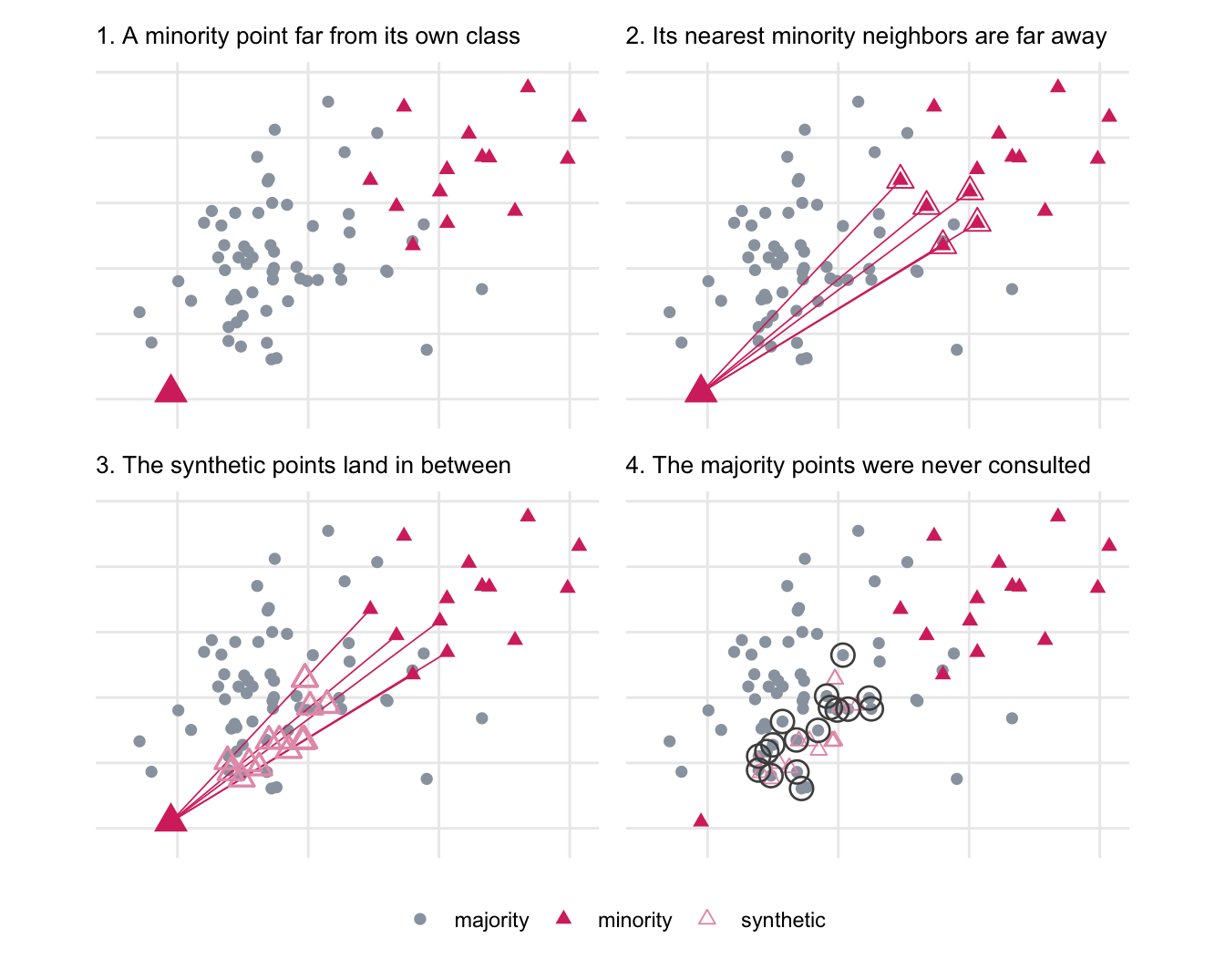
This algorithm has no notion of data quality, meaning that bad data quality can make for some really unfortunate samples, especially for lone outliers. Figure 88.2 follows a single stray minority observation through the same procedure. Its nearest minority neighbors are all the way across the majority class, so the interpolation runs straight through territory where no minority observation was ever seen, and the synthetic points land in the middle of the majority class.
It also treats the observations of each class by itself. While this is computationally and conceptually faster, it is a much simpler data representation, one that doesn’t use any information about their interactions. Furthermore, it includes no information about the majority class, which may otherwise be helpful to guide the method. This is the second thing Figure 88.2 shows: the majority observations in the way of the interpolation are visible to us, but not to the algorithm. Nothing in SMOTE consults them, so nothing stops the bridge from being built.
Since we are using a nearest neighbor search, We have a hyperparameter k that is used to denote how many observations should be considered for pairs.
The nearest neighbor search is central to the SMOTE method and thus responsible for many of the downsides associated with the method. One of the problems is that the idea of nearest neighbors becomes more fuzzy as we enter higher dimensions. This will naturally extend to how SMOTE becomes applicable. Similarly, the nearest neighbor search is also responsible for the high computational cost that can occur when the data becomes larger. computational cost
Many of the different issues are addressed by some of the SMOTE variants.
Base SMOTE needs no expanding to handle more than two classes, as described in Section 86.2.
Like all the methods in this section, this changes the distribution of the training data set, which is covered in Section 86.3.
TipAnimated version
The same walkthrough, one step at a time, is available as an animated slide.
88.2 Pros and Cons
88.2.1 Pros
88.2.2 Cons
88.3 R Examples
We will be using the same subset of the ames data set as in the up-sampling chapter. Note that all the predictors are numeric, which SMOTE requires.
library(recipes)
library(themis)
library(modeldata)
library(dplyr)
data("ames")

ames_imbalance <- ames |>
  filter(MS_Zoning %in% c("Residential_Low_Density", "Residential_Medium_Density")) |>
  mutate(MS_Zoning = droplevels(MS_Zoning)) |>
  select(MS_Zoning, Lot_Area, Year_Built, Gr_Liv_Area, Full_Bath)

ames_imbalance |>
  count(MS_Zoning)
# A tibble: 2 × 2
MS_Zoning n
<fct> <int>
1 Residential_Low_Density 2273
2 Residential_Medium_Density 462{themis} provides step_smote(), which has the implementation for SMOTE.
recipe(MS_Zoning ~ ., data = ames_imbalance) |>
  step_smote(MS_Zoning) |>
  prep() |>
  bake(new_data = NULL) |>
  count(MS_Zoning)
# A tibble: 2 × 2
MS_Zoning n
<fct> <int>
1 Residential_Low_Density 2273
2 Residential_Medium_Density 2273